# Astera 12.0 - Release Notes
This release is a major milestone for Astera, introducing:
* **Astera Cloud** - A comprehensive cloud-native platform that combines our different product offerings into a unified web-based portal. The portal serves as a single hub enabling users to sign up for a personalized experience with our products, download and get started using the right product in the configuration that best fits their needs, and handle administrative tasks such as adding or managing other users. The platform now supports both Dataprep and ReportMiner with scalable cloud infrastructure, dedicated storage, and seamless asset management.
* **Astera Express Editions** - Lightweight versions of our core products designed for faster onboarding and streamlined usage scenarios. These editions remove complexity barriers while maintaining the essential functionality organizations need to get started quickly with data integration and processing tasks.
* **Astera Dataprep** - Our first AI-powered self-service data preparation tool that empowers business users to clean, transform, and prepare their data without requiring technical expertise. This intelligent solution automates complex data preparation tasks while providing an intuitive interface for users at any skill level.
Together, these offerings make it easier than ever for organizations to access, manage, and prepare their data without worrying about infrastructure or complex technical processes. With cloud-native deployments and intuitive data preparation capabilities, this release democratizes data management and processing for organizations of all sizes.
### Astera Cloud
Astera Cloud extends our platform beyond traditional on-premise deployments, allowing teams to leverage the full power of Astera without managing infrastructure. Preconfigured and optimized cloud servers let users focus on designing and running data flows instead of handling server resources.
#### Key Features
* **Lightweight Client Installation:** Install the client designer locally and continue working with the familiar drag-and-drop interface to build data flows, workflows, and more.
* **Server-Side Execution:** All execution, scheduling, and processing runs on managed cloud infrastructure, minimizing local resource usage.
* **Scalable Infrastructure:** Cloud servers automatically adjust to workload demands, ensuring reliable performance without capacity planning.
* **Cloud Storage & Asset Management:** Users receive dedicated cloud storage with easy upload capabilities for flows, source files, and other artifacts from local networks to the cloud environment.
* **Seamless Migration:** Easily migrate existing on-premise flows to the cloud while maintaining compatibility.
With this release, Astera Cloud now supports both Dataprep and ReportMiner, giving users the flexibility to prepare, extract, and integrate data seamlessly in the cloud.

#### Web-Based Management Portal
The Astera Cloud experience is managed through a unified web-based portal that streamlines deployment, administration, and subscription management without the need for lengthy procurement cycles. This single interface provides:
* **User Configuration:** Create and manage accounts with role-based permissions and access controls
* **Client Downloads:** Access and download client applications
The portal provides a seamless experience in managing your complete Astera Cloud experience from one centralized location.

### Astera Express Editions
To simplify onboarding and accelerate adoption, Express editions are now available for both Dataprep and ReportMiner. These lightweight versions are designed for faster setup, simplified usage, and entry-level scenarios.
* **Dataprep Express**: Quick access to AI-powered data preparation for smaller datasets and business use cases.
* **ReportMiner Express**: Streamlined data extraction for simpler scenarios, without the overhead of advanced template management.
By default, the Express editions use local storage, with an option to connect to the cloud
{% hint style="info" %}
**Note:** In the Express editions, you don’t need to run their flows on a server (local or Cloud), as the product itself is designed to handle them at runtime.
{% endhint %}

### Astera Dataprep (New Release)
We are proud to introduce Astera Dataprep, the fastest and simplest way to prepare data for analysis through an AI-powered, chat-based interface. Available on Astera Cloud as well as in the lightweight Dataprep Express edition, it enables both business and technical users to clean, transform, and prepare data by interacting with the AI agent using natural language instructions.
#### Key Features
* **AI-Powered Chat Interface**: Prepare data effortlessly with natural language instructions
* **Preview-Centric Tabular View**: See real-time data changes with every action.
* **Flexible Import and Export Options**: Work with Excel, CSV/TXT, and major databases (SQL Server, Oracle, PostgreSQL).
* **Instant Data Profiling**: Gain insights into data quality, structure, and patterns instantly with real-time graphical profiles and chat-based analysis.
* **Comprehensive Data Operations**: Handle missing values, remove duplicates, fix formatting, and apply transformations through simple natural language instructions.
* **Recipe Mode**: View your data manipulation actions as step-by-step English instructions for clarity and reuse.
* **Workflow Automation (available in Cloud and on-prem client/server)**: Automate preparation processes with scheduled runs and real-time job monitoring.
* **Data Privacy Protection**: Your data remains secure within the Astera platform, no data is ever sent to external LLMs, with the AI used solely to interpret natural language instructions.

This concludes the Astera 12.0 Release Notes.
# Express
# System Requirements
| **Application Processor** | Dual Core or greater *(recommended)*; 2.0 GHz or greater |
| -------------------------------- | ---------------------------------------------------------------------------------------------- |
| **Operating System** | Windows 10 or newer |
| **Memory** | 8GB or greater *(recommended)* |
| **Hard Disk Space** | 2 GB – (*including .NET Desktop Runtime installed)* |
| **AI Subscription Requirements** |
OpenAI API (provided as part of the package)
LLAMA API
Together AI
|
| **Other** | Requires ASP .NET Core 8.0.x Windows and Desktop Runtime 8.0.x |
# Installing Express
In this section we will discuss how to install and configure Astera Dataprep Express.
## How to Install Astera Dataprep Express
1. Run *‘DataprepExpress.exe’* from the installation package to start the express installation setup.
2. Astera Software License Agreement window will appear; check *I agree to the license terms and conditions* checkbox, then click *Install*.
{% hint style="info" %}
**Note:** You can select *Options* to change the default installation directory.
{% endhint %}
3. When the installation is successfully completed, click *Close*.
# Launching Designer
After you have successfully installed Express, open the application and you will see the *User Logon screen* as pictured below.
1. You can skip the log on or proceed with your preferred log on method.
2. Astera offers two methods to create your account:
* *Sign Up with Microsoft* – Useful for users who have an active Microsoft account. No separate sign-up is required, since your Microsoft account already exists and can be used directly for login.
* *Sign Up with Email* – Suitable for any other email domains. In this case, you will have to **Create an account** to complete the account creation process. This step is necessary because Email Authentication requires registration in our Azure tenant. Once created, your email is added both to our database and to the Azure directory.
3. Select your preferred method and go through the MFA steps.
4. Once you have signed up, the designer will launch. You can now start preparing your data.
{% hint style="info" %}
**Note:** You will not be able to use the AI Agent or any AI functionality on the client if you haven’t logged in to your Astera account.
{% endhint %}
### Logging in from the designer
1. To log in from the designer, click the profile dropdown and select *Log in*.
2. This will direct you to a login screen where you can provide your user credentials.
3. After you log in, you can click the *Create New Chat* button in the *Dataprep AI Agent* panel to begin chatting with the agent.
# Cloud
# System Requirements
| **Application Processor** | Dual Core or greater *(recommended)*; 2.0 GHz or greater |
| --------------------------------- | ------------------------------------------------------------------------------------------ |
| **Operating System** | Windows 10 or newer |
| **Memory** | 8GB or greater *(recommended)* |
| **Hard Disk Space** | 2 GB – (*including .NET Desktop Runtime installed)* |
| **AI Subscription Requirements** |
OpenAI API
LLAMA API
Together AI
|
| **OCR Subscription Requirements** |
Tesseract (Provided as part of the package) Google OCR Amazon Textract
|
| **Other** | Requires ASP .NET Core 8.0.x Windows and Desktop Runtime 8.0.x |
# Creating an Account in Astera Cloud Portal
The Astera Cloud Portal provides secure access for managing your data integration projects in the cloud. In this document, we will walk through the steps to create an account on the Cloud Portal.
1. Go to [cloudastera.com](https://cloudastera.com/).
2. Click *Create an account*.
3. Astera offers two methods to create your account:
* *Sign Up with Microsoft* – Useful for users who have an active Microsoft account.
* *Sign Up with Email* – Suitable for any other email domains.
Select your preferred method and go through the MFA steps.
4. Once you have signed up, Step 2: *Profile* will appear. Enter your *First Name* and *Last Name* here.
5. Click *Start Trial,* you will be directed to the portal home page
You can now launch your designer by clicking *Launch Designer* to start designing data integration flows in Astera.
# Launching Designer
Data pipelines in Astera, are designed in the Designer. The designer is a desktop based interface where users can design and test their pipelines before they run them on the cloud server.
1. To get started, you need to launch your designer from the portal by clicking on *Launch Designer.*

2. The launch designer screen will appear, which will automatically open the designer if previously downloaded. If not, download it by clicking the *Download* button.

3. The download button will download an executable, run the executable.
4. Astera Software License Agreement window will appear; check *I agree to the license terms and conditions* checkbox, then click *Install*.
{% hint style="info" %}
**Note:** You can select *Options* to change the default installation directory.
{% endhint %}
5. When the installation is successfully completed, click *Close*.
6. The designer will now launch automatically.
The designer has successfully launched; you can now start preparing your data.
# User Management
Managing user access in Astera Cloud Portal is user-centric and allows you to efficiently control who can access your cloud resources. This guide will walk you through the process of managing users in your Organization.
### User Management
1. Let's begin by navigating to the *User Management* section in your Astera Cloud Portal.\
Here, you'll see the *User Management* interface displaying existing users and their roles
2. To add a new user to your portal, click on the *Invite User* button.
3. The *Add User* pop-up will appear. Here, you'll need to provide the following information:
* Email Address: Enter the email address of the user you want to invite
* Role Assignment: You can assign one of two roles to the new user:
* Admin: Provides full administrative access to the portal, including the ability to manage other users, access all resources, and modify settings
* User: Provides standard user access with limited administrative privileges
* Click *Send Invite* to send an invitation email to the new user. A success message will appear notifying if the email was sent successfully.
The user will now be able to accept the invitation and login to this organization.
{% hint style="info" %}
**Note:** The invitation is only valid for 3 days, if the user could not accept the invitation within the time limit, then you can resend the invitation.
{% endhint %}
### Managing Invitations
After sending an invitation, you can monitor the status of your invites in the *Invited* section.

The interface displays several important details about each user:
* Email: The user's email address
* Roles: Displays the assigned role (Admin or User)
* Status: Shows whether the user is *Active*, *Accepted* or *Cancelled*
* Active: The invitation has been sent but not yet accepted
* Accepted: The user has accepted the invitation and can access the portal
* Cancelled: The invitation for the user has been cancelled
* Actions:
* Cancel Invitation: Cancel an invitation here.
* Resend Invitation: Resend an invitation here
### Managing Existing Users
Once users have accepted their invitations and are part of your organization, an *Admin* can manage their access and roles as needed in the *Users* section.
In the *Actions* column for each active user, you'll find a menu with the following options:
* Delete: Permanently removes the user from the organization
* Deactivate: Temporarily disables the user's access without removing them
* Make Admin: Promotes a regular user to admin role
# Managing Files and Folders in Designer
Astera Cloud allows you to seamlessly transfer content between your local machine and the cloud environment. Whether bringing local files into Astera Designer or saving work back to your system, the Designer offers intuitive tools for efficient content management. This document explains how to perform both upload and download operations.
{% tabs %}
{% tab title="Uploading Content" %}
### Using the Toolbar Option
You can upload files using the Upload button in the tool-bar or by pressing Ctrl + U on the keyboard.

This button also has a dropdown option to *Upload Folder* if you want to upload an entire folder instead of individual files.

Your local file explorer will open. Here you can select the files (or folder if using the dropdown option) you want to upload and click *Open*.
A success message will appear and the *Data Source Browser* panel will open with the uploaded content in a *Default Uploads* folder.
### Using the *Data Source Browser* panel
The *Data Source Browser* panel also has a similar upload button . This option will only be enabled when a user has selected a folder, as this button is designed to upload files or folders to the selected folder rather than the *Default Folder*. The rest of the steps remain the same as before.
{% endtab %}
{% tab title="Downloading Content" %}
To save files or folders from Astera Cloud to your local machine, you can use the download functionality available in the Designer.
In this document, we will learn how to download files and folders from the Designer.
### Using the Data Source Browser Panel
1. You can download content by first selecting a file or folder in the *Data Source Browser* panel, this will enable the *Download* button.
2. Click the *Download* button.
3. Your local file explorer will open, allowing you to choose where you want to save the downloaded content. Select your preferred download location and click OK.\
The selected content will be downloaded to your chosen location.
4. Once the download is complete, a success message will appear confirming that the download was successful.
{% endtab %}
{% endtabs %}
# On Prem
# System Requirements
| **Client Application Processor** | Dual Core or greater *(recommended)*; 2.0 GHz or greater |
| --------------------------------- | ------------------------------------------------------------------------------------------------------------------------------------------------------------- |
| **Server Application Processor** | 8 Cores or greater *(recommended)* |
| **Repository Database** |
MS SQL Server 2008R2 or newer, or PostgreSQL v15 or newer for hosting repository database
|
| **Operating System - Client** | Windows 10 or newer |
| **Operating System - Server** | **Windows:** Windows 10 or Windows Server 2019 or newer |
| **Memory** | **Client:** 8GB or greater *(recommended)* |
| |
Server: 8GB or greater (recommended)
32GB or greater for large data processing
32GB or greater for AI processing
|
| **Hard Disk Space** | **Client:** 2GB– *(if .NET Framework is pre-installed)* |
| | **Server:** 2GB – (if .NET Framework is pre-installed) |
| | *Additional 300 MB if .NET Framework is not installed* |
| **AI Subscription Requirements** |
OpenAI API
LLAMA API
Together AI
Postgres Db (if knowledgebase is needed)
|
| **OCR Subscription Requirements** |
Tesseract (Provided as part of the package) Google OCR Amazon Textract
|
| **Other** |
Requires ASP.NET Core 8.0.x Windows and Desktop Runtime 8.0.x for the client,
.NET Core Runtime 8.0.x for the server
|
{% hint style="info" %}
**Note**: The overall speed and performance of the application depend on the configuration of your machine. More memory and higher processing speed on the system will result in faster performance, especially when transferring large amounts of data as the application takes advantage of the multicore hardware to parallelize operations.
{% endhint %}
# Product Architecture
Astera Data Stack is built on a client-server architecture. The client is the part of the application which a user can run locally on their machine, whereas the server performs processing and querying requested by the client. In simple words, the client sends a request to the server, and the server, in turn, responds to the request. Therefore, database drivers are installed only on the Astera Data Stack server. This enables horizontal scaling by adding multiple clients to an existing cluster of servers and eliminating the need to install drivers on every machine.
The Astera client and server applications communicate on REST architecture. REST-compliant systems, often called RESTful systems, are characterized by statelessness and separate concerns of the client and server, which means that the implementation of both can be done independently if each side knows what format of messages to send to the other. The server communicates with the client using HTTPS commands, which are encrypted using a certified key/certificate signed by an authority. This saves the data from being intercepted by an attacker as the plaintext is encrypted as a random string of characters.
# Installing Client and Server Applications
In this section we will discuss how to install and configure Astera Server and Client applications.
## How to Install Astera Server
1. Run *‘IntegrationServer.exe’* from the installation package to start the server installation setup.
2. Astera Software License Agreement window will appear; check *I agree to the license terms and conditions* checkbox, then click *Install*.
{% hint style="info" %}
**Note:** You can select *Options* to change the default installation directory and server port.
{% endhint %}
3. Your server installation has been completed. If you want to use advanced features such as OCR, Text Converter, etc, click on *Install Python Server* and follow the steps [here](/setting-up/on-prem/install-manager/installing-packages-on-server-machine)*.*
## How to install Astera Client
1. Run the *‘ReportMiner’* application from the installation package to start the client installation setup.
2. Astera Software License Agreement window will appear; check *I agree to the license terms and conditions* checkbox, then click *Install*.
{% hint style="info" %}
**Note:** You can select *Options* to change the default installation directory.
{% endhint %}
3. When the installation is successfully completed, click *Close*.
***
# Install Manager
In order for advanced features such as AGL, OCR and Text Converter to work in Astera, different packages are required to be installed, such as Python, Java etc. To avoid the tedious process of separately installing these, Astera provides a built in Install Manager in your tool.
There are two types of packages which are required to be installed:
* Prerequisites for Python Server: This package is required to be installed on server machine only.
* Prerequisites for ReportMiner: This package is required to be installed on client and server machine.
{% hint style="info" %}
**Note:** If the server and client are on same machine, then ReportMiner packages need to be installed once only.
{% endhint %}
The packages being installed for AGL are listed as follows:
* [Java 17](https://www.oracle.com/java/technologies/downloads/#jdk17-windows) is installed
* [Python 3.9.7](https://www.python.org/ftp/python/3.9.7/python-3.9.7-amd64.exe) with the following packages:
* [Tabula-py](https://pypi.org/project/tabula-py/)
* [Tabulate](https://pypi.org/project/tabulate/)
* [spaCy](https://spacy.io/usage/spacy-101)
* [NLP](http://www.cse.unsw.edu.au/~billw/nlpdict.html)
The packages being installed for OCR are listed as follows:
* [Python 3.9.7](https://www.python.org/ftp/python/3.9.7/python-3.9.7-amd64.exe)
* [ImageMagicK](https://imagemagick.org/archive/binaries/ImageMagick-7.1.0-43-Q16-HDRI-x64-dll.exe)
* [Tesseract](https://digi.bib.uni-mannheim.de/tesseract/tesseract-ocr-w64-setup-v5.1.0.20220510.exe)
* Python packages
* [commandline](https://pypi.org/project/commandline/0.1.3dev/)
* [fpdf](https://pypi.org/project/fpdf/)
* [minecart](https://pypi.org/project/minecart/)
* [numpy](https://pypi.org/project/numpy/1.20.3/)
* [opencv-contrib-python](https://pypi.org/project/opencv-contrib-python/4.5.3.56/)
* [opencv-python](https://pypi.org/project/opencv-python/4.5.2.52/)
* [packaging](https://pypi.org/project/packaging/20.9/)
* [pandas](https://pypi.org/project/pandas/1.2.4/)
* [pathlib](https://pypi.org/project/pathlib/)
* [pdf2image](https://pypi.org/project/pdf2image/1.15.1/)
* [Pillow](https://pypi.org/project/Pillow/8.2.0/)
* [py2exe](https://pypi.org/project/py2exe/0.10.4.1/)
* [PyMuPDF](https://pypi.org/project/PyMuPDF/1.18.19/)
* [PyPDF2](https://pypi.org/project/PyPDF2/1.26.0/)
* [pyreadline](https://pypi.org/project/pyreadline/)
* [pytesseract](https://pypi.org/project/pytesseract/0.3.7/)
* [pytessy](https://pypi.org/project/pytessy/)
* [regex](https://pypi.org/project/regex/2021.4.4/)
* [scikit-learn](https://pypi.org/project/scikit-learn/0.24.2/)
* [tesseract](https://pypi.org/project/tesseract/)
* [threadpoolctl](https://pypi.org/project/threadpoolctl/2.1.0/)
* [openpyxl](https://pypi.org/project/openpyxl/3.0.10/)
* [scipy](https://pypi.org/project/scipy/1.8.1/)
* [pikepdf](https://pypi.org/project/pikepdf/5.4.0/)
* [wand](https://pypi.org/project/Wand/0.6.8/)
The packages being installed for Python Server are listed as follows:
* Python Server executable is installed (comes with all packages necessary for Python Server)
* [ffmpeg](https://www.bing.com/ck/a?!&\&p=adc30574394062132875268546616bca253dc3ed7740cd89374c712cc221b05aJmltdHM9MTc0Mjc3NDQwMA\&ptn=3\&ver=2\&hsh=4\&fclid=053b0a9d-97ef-68f5-0a5f-1e9a965b69fb\&psq=ffmpeg\&u=a1aHR0cHM6Ly9mZm1wZWcub3JnL2Rvd25sb2FkLmh0bWw\&ntb=1)
* [ImageMagicK](https://imagemagick.org/archive/binaries/ImageMagick-7.1.0-43-Q16-HDRI-x64-dll.exe)
* [Tesseract](https://digi.bib.uni-mannheim.de/tesseract/tesseract-ocr-w64-setup-v5.1.0.20220510.exe)
* [Java 17](https://www.oracle.com/java/technologies/downloads/#jdk17-windows) is installed
In the following documents, we will look at how to use the install manager to install these packages on client and server machines.
# Installing Packages on Client Machine
1. Open Astera as an administrator.
2. Once Astera is open, go to the *Tools > Run Install Manager*.
3. The Install Manager welcome window will appear. Click on *Next*.
4. If the prerequisite packages are already installed, the Install Manager will inform you about them and give you the option to uninstall or update them as needed.
5. If the prerequisite packages are not installed, then the Install Manager will present you with the option to install them. Check the box next to the pre-requisite package, and then click on *Install*.
{% hint style="info" %}
Note: If your client and server are on the same machine, then you can also install Python Server directly at this stage.
{% endhint %}
6. During the installation, the Install Manager window will display a progress bar showing the installation progress.
You can also cancel the installation at any point if necessary.
7. Once the installation is complete, the Install Manager will prompt you. Click on *Close* to exit out of the Install Manager.
The packages for AGL and OCR usage are now installed, and the features are ready to use.
{% hint style="info" %}
**Note:** The packages are ready to use in the case when both the Integration Server and Astera are installed on the same machine.
{% endhint %}
In case the Integration Server is installed on a separate machine, we will need to install the packages for AGL and OCR there as well.
# Installing Packages on Server Machine
1. In order to access the install manager on the sever machine, open start and search for “Install Manager for Integration Server”.
2. Run this Install Manager as admin.
3. The Install Manager welcome window will appear. Click on *Next*.
4. If the prerequisite packages are already installed, the Install Manager will inform you about them and give you the option to uninstall or update them as needed.
5. If the prerequisite packages are not installed, then the Install Manager will present you with the option to install them. Check the box next to the pre-requisite package, and then click on *Install*.
6. During the installation, the Install Manager window will display a progress bar showing the installation progress.
You can also cancel the installation at any point if necessary.
7. Once the installation is complete, the Install Manager will prompt you. Click on *Close* to exit out of the Install Manager.
This concludes our discussion on how to use the install manager for Astera.
# Connecting to an Astera Server using the Client
{% embed url="" %}
### How to connect to an Astera Server from the Client Startup Screen
After you have successfully installed Astera client and server applications, open the client application and you will see the *Server Connection* screen as pictured below.
Enter the *Server URI* and *Port Number* to establish the connection.
The server URI will be the IP address of the machine where Astera Integration server is installed.
*Server URI:* ()
{% hint style="info" %}
**Note:** You can get help of your network administrator to get the IP address of the machine where Astera Integration server is installed. Or you can launch the command prompt and type the command *ipconfig* to get the IP configuration details for the machine and use that information to provide Server URI.
{% endhint %}
The default port for the secure connection between the client and the Astera Integration server is 9264.
If you have connected to any server recently, you can automatically connect to that server by selecting that server from the *Recently Used* drop-down list.
Click *Connect* after you have filled out the information required.
The client will now connect to the selected server. You should be able to see the server listed in the *Server Explorer* tree when the client application opens.
To open *Server Explorer* go to *Server > Server Explorer* or use the keyboard shortcut **Ctrl + Alt + E**.
Before you can start working with the Astera client, you will have to create a repository and configure the server.
# How to Connect to a Different Astera Server from the Client
{% embed url="" %}
You can connect to different servers right from the Server Explorer window in the Client. Go to the *Server Explorer* window and click on the Connect to Server icon.
A prompt will appear that will confirm if you want to disconnect from the current Server and establish connection to a different server. Click *Yes* to proceed.
{% hint style="info" %}
**Note:** A client cannot be connected to multiple servers at once.
{% endhint %}
You will be directed to the *Server Connection* screen. Enter the required server information (Server URI and Port Number) to connect to the server and click *Connect*.
If the connection is successfully established, you should be able to see the connected server in the Server Explorer window.
# How to Build a Cluster Database and Create Repository
Before you start using the Astera server, a repository must be set up. Astera supports SQL Server and PostgreSQL for building cluster databases, which can then be used for maintaining the repository. The repository is where job logs, job queues, and schedules are kept.
To see these options, go to *Server > Configure > Step 1: Build repository database and configure server*.
The first step is to point to the SQL Server or PostgreSQL instance where you want to build the repository and provide the credentials to establish the connection.
{% hint style="info" %}
**Note:** Astera will not create the database itself, just the tables. A database will have to be created beforehand or an existing database can be used. We recommend Astera to have its own database for this purpose.
{% endhint %}
### Building a Repository on SQL Server
1. Go to *Server > Configure > Step 1: Build repository database and configure server*.
2. Select SQL Server from the Data Provider drop-down list and provide the credentials for establishing the connection.
3. From the drop-down list next to the Database option, select the database on the SQL instance where you want to host the repository.
4. Click *Test Connection* to test whether the connection is successfully established or not. You should be able to see the following message if the connection is successfully established.
4. Click *OK* to exit out of the test connection window and again click *OK*, the following message will appear. Select *Yes* to proceed.
The repository is now set up and configured with the server to be used.
The next step is to log in using your credentials.
### Building a Repository on PostgreSQL
1. Go to *Server > Configure > Step 1: Build repository database and configure server*.
2. Select PostgreSQL from the Data Provider drop-down list and provide the credentials for establishing the connection.
3. From the drop-down list next to the *Database* option, select the database on the PostgreSQL instance where you want to host the repository.
4. Click *Test Connection* to test whether the connection is successfully established or not. You should be able to see the following message if the connection is successfully established.
5. Click *OK* and the following message will appear. Select *Yes* to proceed.
The repository is now set up and configured with the server to be used.
The next step is to log in using your credentials.
# Repository Upgrade Utility in Astera
Existing Astera customers can upgrade to the latest version of Astera Data Stack by executing an exe. script, which automates the repository update to the latest release. This streamlined approach enhances the efficiency and effectiveness of the upgrade process, ensuring a smoother transition for users.
{% hint style="info" %}
**Note:** This upgrade applies to v10.0 and later ones. Previous versions cannot be upgraded and will need a clean repository as part of the upgrade.
{% endhint %}
1. To start, download and run the latest server and client installers to upgrade the build.
{% hint style="info" %}
Note: Depending on the build, the user can upgrade any of the respective client and server.
{% endhint %}
2. Run the Repository Upgrade Utility to upgrade the repository.
{% hint style="info" %}
**Note:** If you do not perform this step, you might encounter an error.
{% endhint %}
3. Once run, you will be faced with the following prompt.
Click *OK* and the repository will be upgraded.
Once done, you will be able to view all jobs, schedules, and deployments that you previously worked with in the Job Monitor, Scheduler, and Deployment windows.
This concludes the working of the Repository Upgrade Utility in Astera Data Stack.
# How to Login from the Client
Once you have created the repository and configured the server, the next step is to login using your Astera account credentials.
You will not be able to design any dataflows or workflows on the client if you haven’t logged in to your Astera account. The options will be disabled.
### Log in to your user account
1. Go to *Server > Configure > Step 2: Login as admin*.
2. This will direct you to a login screen where you can provide your user credentials.
If you are using Astera 10 for the first time, you can login using the default credentials as follows:
*Username: admin* *Password: Admin123*
After you log in, you will see that the options in the Astera Client are enabled.
You can use these options until your trial period is active. For fully activating the options and the product, you’ll have to enter your license.
### How to automatically reconnect on client startup
If you don’t want Astera to show you the server connection screen every time you run the client application, you can skip that by modifying the settings.
To do that go to **Tools > Options > Client Startup** and select the *Auto Connect to Server* option. On enabling the option, Astera will store the server details you entered previously and will use those details to automatically reconnect to the server every time you run the application.
The next step after logging in is to unlock Astera using the License key.
# How to Verify Admin Email
Once you have logged into the Astera client, you can set up an admin email to access the Astera server. This will also allow you to be able to use the “*Forgot Password*” option at the time of log in.
In this document, we will discuss how to verify admin email in Astera.
### Verifying Admin Email
1\. Once logged in, we will now proceed to enter an email address to associate with the admin user by verifying the email address.
Go to *Server > Configure > Step 3: Verify Admin Email*
2\. Unless you have already set up an email address in the *Mail Setup* section of *Cluster settings,* the following dialogue box will pop up asking you to configure your email settings.
Click on *Yes* to open your cluster settings.
Click on the *Mail Setup* tab.
3\. Enter your email server settings.
4\. Now, right-click on the Cluster Settings active tab and click on *Save & Close* in order to save the mail setup.
5\. Re-visit the *Verify Admin Email* step by going to *Server > Configure > Step 3: Verify Admin Email*.
This time, the *Configure Email* dialogue box will open.
6\. Enter the email address you previously set up and click on *Send OTP*.
7\. Use the OTP from the email you received and enter it in the *Configure Email* dialogue and proceed.
On correct entry of the OTP, an email successfully configured dialogue will appear.
8\. Click *OK* to exit it. We can confirm our email configuration by going to the *User List*.
Right click on *DEFAULT* under *Server Connections* in the *Server Explorer* and go to *User List*.
9\. This opens the *User List* where you can confirm that the email address has been configured with the admin user.
### Using Forgot Password feature
The feature is now configured and can be utilized when needed by clicking on *Forgot Password* in the log in window.
This opens the *Password Reset* window, where you can enter the OTP sent to the specified e-mail for the user and proceed to reset your password.
This concludes our discussion on verifying admin email in Astera.
# Licensing in Astera
{% embed url="" %}
### Single license key model
The license key provided to you contains information about how many Astera clients can connect to a single server as well as the functionality available to the connected clients.
{% hint style="info" %}
**Note**: You cannot use your existing set of keys (from version 6 or 7). If you are planning to migrate from version 7 (or earlier) to version 8, 9 or 10, please contact [sales@astera.com](mailto:sales%40astera.com), as you will need a new license key.
{% endhint %}
### Unlocking Astera using your license key
After you have configured the server, and logged in with the admin credentials, the last step is to insert your license key.
1. Go to *Server > Configure > Step 4: Enter License Key*.
2. On the License Management window, click on *Unlock using a key.*
3. Enter the details to unlock Astera – Name, Organization, and Product Key and select *Unlock.*
4. You’ll be shown the message that your license has been successfully activated.
{% hint style="info" %}
**Note:** The connected client applications will shut down for the server license to take effect.
{% endhint %}
Your client is now activated. To check your license status, you can go to *Tools > Manage Server License*.
This opens a window containing information about your license.
This concludes unlocking Astera client and server applications using a single licensing key.
# How to Supply a License Key Without Prompting the User
In some cases, it may be necessary to supply a license key without prompting the end user to do so. For example, in a scenario where the end user does not have access to install software, a systems administrator may do this as part of a script.
One possible solution is to place the license key in a text file. This way, the administrator can easily license each machine without having to go through the licensing prompt for each user.
Here’s a step-by-step guide to supplying a license key without prompting the user:
### **Step 1: Create a** **New Text Document**
To get started, create a new text document that will hold the license key required to access the application.
### **Step 2: Enter the License Key**
In the text document, enter a valid license key. The key must be the only thing in the document, and it must be on the very first line. Make sure there are no unnecessary leading or trailing spaces, lines, or any characters other than those of the license key.
### **Step 3: Save the Text Document by the name “Serial” in the Server Application Folder**
Name the text document “Serial” and save it in the Integration Server Folder of the application located in Program Files on your PC. For instance, if the application is Astera, save the Text Document in the “Astera Integration Server 10” folder. This folder contains the files and settings for the server application. The directory path would be as follows:
*C:\Program Files\Astera Software\Astera Integration Server 10.*
{% hint style="info" %}
**Note:** This approach works for all Astera applications, except for Astera API Management and Astera Express. For API Management, there is a different server. Thus, for it, you’ll need to locate the corresponding server folder and follow the same steps. Whereas for Astera Express, since there is no server involved, simply copy the *Serial* text document to the “Astera Express 10” folder, and the remaining steps remain unchanged.
{% endhint %}
### **Step 4: Restart the Service**
Finally, restart the *Astera Integration Server 10* service to complete the process. This step ensures that, from now on, when the user launches Astera or any other application by Astera, they will not be prompted to enter a license key.
{% hint style="info" %}
**Note:** There is no need to restart the service for Astera Express as it does not have a corresponding server.
{% endhint %}
Also, please keep in mind that all license restrictions are still in effect, and this process only bypasses the user prompt for the key.
In conclusion, by following these simple steps, system administrators can easily supply a license key without prompting the end user. This approach is particularly useful when installing software remotely or when licensing multiple machines.
# Enabling Python Server
The Python server is embedded in the Astera server and is required to use the Text Converter object in the tool. It is disabled by default, and this document will guide us through the process of enabling it.
## Steps
1. Launch the client and navigate to *Server > Manage > Server Properties*.
2. In the Server Properties, check the *Start Python Server* checkbo*x* and press *Ctrl + S* to save your changes.
3. Now open the *Start Menu > Services* and restart the service of Astera Integration Server 11.1.
4. After restarting the service, wait for a few minutes and run cmd as administrator.
5. Type**`netstat -ano | findstr :5001`** command in the command prompt to check if your python server is running.
We’ve successfully enabled the Python server. You can now close this window and use any python server dependent features in the Client.
# User Roles and Access Control
This article introduces the role-based access control mechanism in Astera. This means that administrators can grant or restrict access to various users within the organization, based on their role in the entire data management cycle.
{% embed url="" %}
In this article, we will look at the user lists and role management features in detail.
### How to Create a New User
{% hint style="info" %}
**Note:** When you run the application for the first time, sign in using the default credentials provided on our help site.
{% endhint %}
Username: admin
Password: Admin123
Once you have logged in, you now have the option to create new users and we recommend you to do this as a first step.
1. To create/register a new user, right-click on the DEFAULT server node in the Server Explorer window and select *User List* from the context menu.
This will open the Server Browser panel.
2. Under the *Security* node, right-click on the *User* node and select *Register User* from the context menu.
This will open a new window. You can see quite a few fields required to be filled here to register a new user.
{% hint style="info" %}
**Note:** Astera currently supports three authentication types when registering a user; Astera, Windows, and Azure Authentication.
{% endhint %}
3. Once the fields have been filled, click *Register* and a new user will be registered.
### How to Assign User Roles
Now that a new user is registered, the next step is assign roles to the user.
1. Select the user you want to assign the role(s) to and right-click on it. From the context menu, select *Edit User Roles*.
A new window will open where you can see all roles that are there by default in Astera or are custom created. We haven’t created any custom role, so we’ll see the three default roles that are - *Developer*, *Operator*, and *Root*.
2. Select the role that you want to assign to the user and click on the arrows in the middle section of the screen. You’ll see that the selected role will get transferred from the *All Roles* section to the *User Roles* section.
{% hint style="info" %}
**Note:** You can assign multiple roles to a single user.
{% endhint %}
3. After you have assigned the roles. click OK and the specific role(s) will be assigned to the user.
### Managing Role Resources
Astera lets the admin manage resources allowed to any user. They can assign permissions of resources or they can restrict resources.
1. To edit role resources, right-click on any of the roles and select *Edit Role Resources* from the context menu.
This will open a new window. Here, you can see four nodes on the left under which resources can be assigned,
The admin can provide a role with resources from the *Url* node, the *Cmd* node, access to deployments from the *REST* node and access to Catalog aritfacts from the *Catalog* Node.
Expanding the *Url* node shows us the following resources,
Expanding the *Cmd* node will give us the following checkboxes as resources.
If we expand the REST *checkbox, we can see a list of available API resources, including endpoints you might have deployed.*
Upon expanding the *Catalog* node, we can see the artifacts that have been added to the Catalog, along with which endpoint permissions are to be given.
This concludes User Roles and Access Control in Astera Data Stack.
# Windows Authentication
Windows authentication is a security feature that allows users to log into a system using their Windows credentials.
Astera Data Stack leverages this authentication method and provides the option to register new users using Windows authentication through its Server Browser interface.
### Configuring LDAP path
Before a new user can be registered through the security section of the Server Browser, the LDAP path needs to be configured.
1. To start, right-click on the server’s name node and select *Cluster Settings* from the context menu.

This will open a new window.

2. Click on the LDAP path and provide the LDAP path.
The LDAP path is the IP address provided by the user from where authentication is being done.

Once done, save and close the *Cluster Settings* window.
### Registering user using Windows Authentication
1. To register a user using Windows Authentication, open the security filter of the Server Browser.

2. Right Click on Users and Select *Register User*

This will open a new window.
3. Select *Windows Authentication* from the *Registration* drop-down menu.

4. After selecting Windows Authentication, a new screen will appear in which the server is retrieving a list of users.

5. Here, you can see a search bar and a grid with a column of *User Email Id*

There are two ways to specify the user we want to register.
#### Search bar dropdown
Here, we can specify a user by selecting from the dropdown given in the textbox of the search bar.
{% hint style="info" %}
**Note:** The drop-down will get the list of users that exist in that active directory.
{% endhint %}

#### Manual Search
We can also fetch a user by using the search textbox to look for a specific user.
Clicking on the user will select them.

6. After the user has been selected, the email id will be displayed in the grid of *User Email Id*.

7. Click Register and we can see that the selected users have been added.

The users can now be activated or assigned roles, as is the current way in Astera.
{% hint style="info" %}
**Note:** Users that have been registered using windows authentication can only be activated, deactivated, and deleted.
{% endhint %}
#### Login Using Windows Authentication
Once users have been registered with Windows authentication, they can login with the same authentication credentials.
To log in, select the *Log In* option from the top right of the client window.

Selecting this will open a new window.
In the authentication Dropdown, there are three options:
1. *Centerprise*: For Users that are created by using a simple/existing registration method.
2. *Windows Authentication:* For users that are created by using the Windows authentication method.
3. *Azure Authentication:* For users that are created using the Azure authentication method
By Selecting Windows Authentication, It will autofill the username and lock both text boxes.

{% hint style="info" %}
**Note:** If a user is activated, then they can click directly on *Log* *In*, and they will log in without entering any additional information.
{% endhint %}
This concludes the working of Windows Authentication in Astera Data Stack.
# Azure Authentication
Azure authentication is a security feature that allows users to log into a system using their Microsoft Azure credentials.
Astera Data Stack leverages this authentication method and provides the option to register new users using Azure authentication through its Server Browser interface.
## **Configuring Azure Authentication Credentials**
1. Go to *Server > Cluster > Cluster Settings*
2. Click on Authentication mode tab and select Azure Authentication from dropdown
3. Provide a valid *Client Id*, *Redirect URI* and *Account Type*
{% hint style="info" %}
**Note:** You can find your *Client ID, Redirect URI* and *Account Type* in you Azure Portal.
{% endhint %}

## **Registering user using Azure Authentication**
1. After Configuring Azure Credentials, navigate to *Server Browser* tool window by pressing ctrl + alt + B*.*
2. Here, in *Security > User*, right-click on *User* and select **Register User**

3. A *Register User* window will open, in the *Registration* drop-down select **Azure Authentication**

4. Once selected, Astera will start retrieving a list of users.

5. Once the users have been retrieved, a search UI will appear.

Now there are two ways to specify user you want to register
* By clicking on the dropdown given in the search bar, this will show the list of all users which exist in that active directory:

* By just directly searching in the search bar for a specific user and clicking **e*****nter*** so that user will be selected:

6. Once the user has been selected by one of the methods, the selected email id will be displayed in a *User Email Id* grid.

7. Now Click Register and you can see that selected users added

8. Now you can [activate them or assign them a role](https://documentation.astera.com/latest/setting-up/user-roles-and-access-control) as you would normally do in Astera
{% hint style="info" %}
**Note:** Users Registered using azure authentication can only activated, deactivated, or deleted
{% endhint %}
## **Login Using Azure Authentication**
Once users have been registered with Azure authentication, they can login with the same authentication credentials.
1. To log in, select the *Log In* option from the top right of the client window.
Selecting this will open a new window.
In the authentication Dropdown, there are three options:
* *Centerprise*: For Users that are created by using a simple/existing registration method.
* *Windows Authentication:* For users that are created by using the Windows authentication method.
* *Azure Authentication:* For users that are created using the Azure authentication method

2. By selecting Azure Authentication, the email and password textbox will get locked. Click on *Log In*

3. User would be redirected to the Microsoft sign-in screen where they can sign-in as they would normally do with their email id and password.

This concludes the working of Azure Authentication in Astera Data Stack.
# Offline Activation of Astera
To activate Astera on your machine, you need to enter the license key provided with the product. When the license key is entered, the client sends a request to the licensing server to grant the permission to connect. This action can only be performed when the client machine is connected to the internet.
However, Astera provides an alternative method to activate the license offline by providing an activation code to the users who request for it. Follow the steps given below for offline activation:
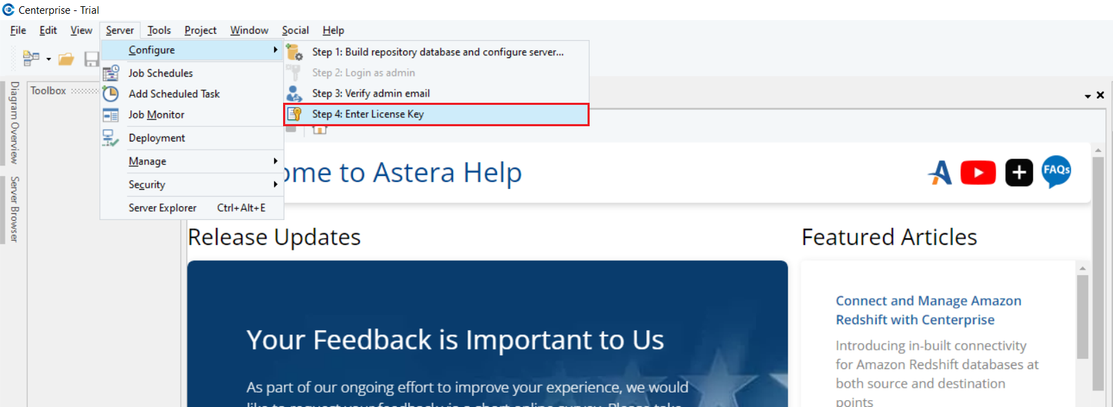
1\. Go to the menu bar and click on *Server > Configure > Step 4: Enter License Key*
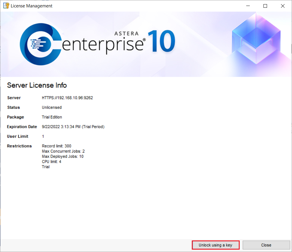
2\. Click on *Unlock using a key.*
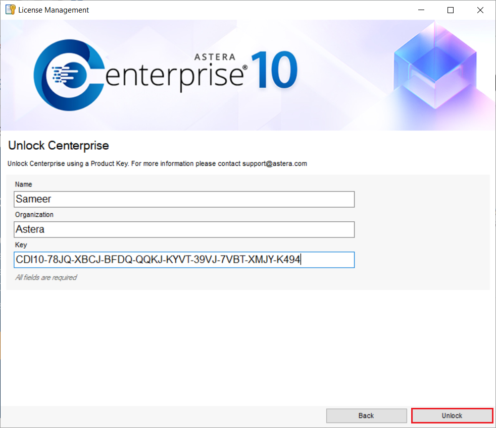
3\. Type your *Name*, *Organization* and paste the *Key* provided to you. Then, click *Unlock*. Do the same if you are changing (instead of activating) your license offline.
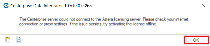
4\. Another pop-up window will give you an error about the server being unavailable because you cannot connect to the server offline. Click *OK.*
5\. Click on *Activate using a key* button.
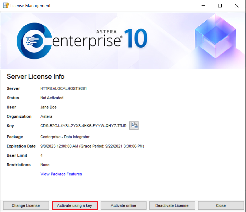
6\. Now, copy the *Key* and the *Machine Hash* and email it to [support@astera.com.](mailto:support%40astera.com) The *Machine Hash* is unique for every machine. Make sure you send the correct *Key* and *Machine Hash* as it is very important for generating the correct *Activation* *Code*.
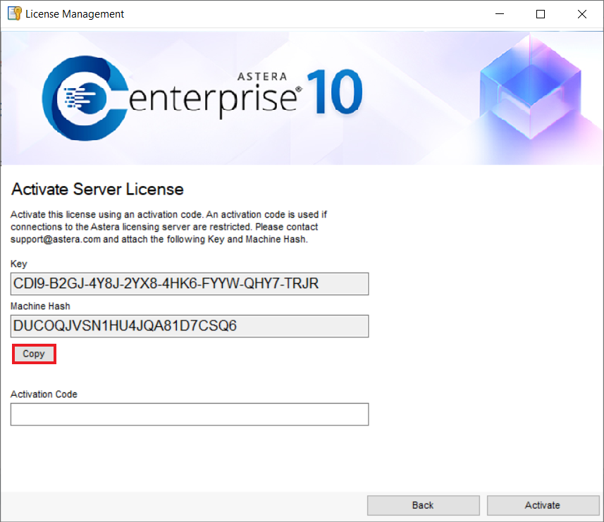
7\. You will receive an activation code from the support staff via e-mail. Paste this code into the *Activation Code* textbox and click on *Activate.*
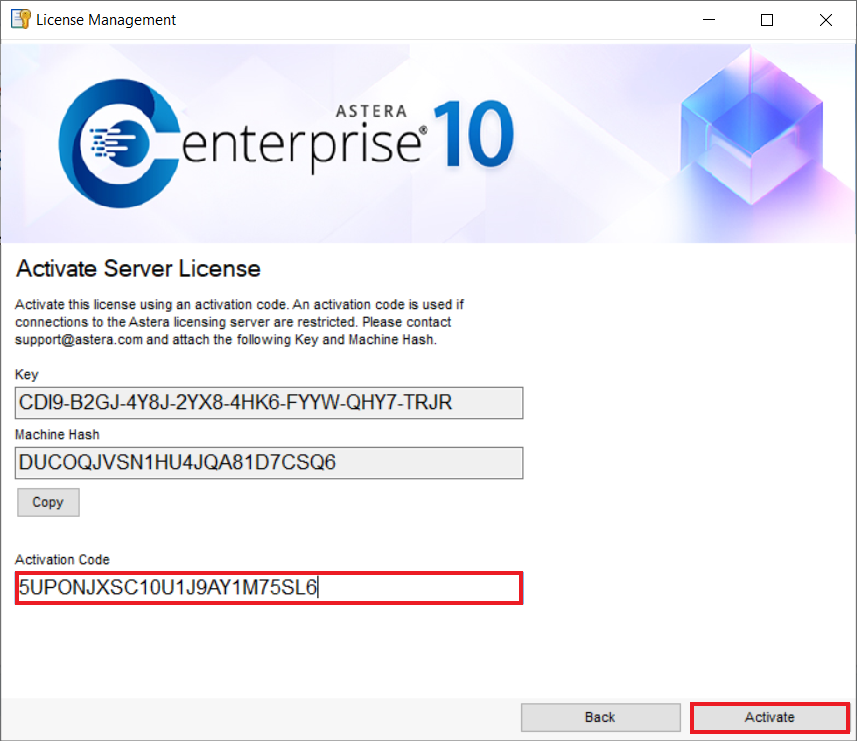
8\. You have successfully activated Astera on your machine offline using the activation code. Click *OK*.
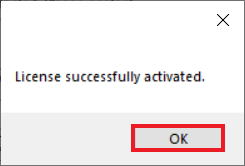
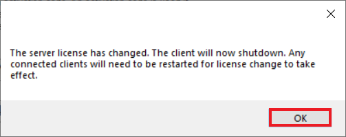
9\. A pop-up window will notify you that the client needs to restart for the new license to take effect. Click *OK* and restart the client.
You have successfully completed the offline activation of Astera.
# Silent Installation
### What is Silent Installation?
Silent installation refers to the installation of software or applications on a computer system without requiring any user interaction or input. In a silent installation, the installation process occurs in the background, without displaying any user interfaces, prompts, or dialog boxes that would normally require the user to make choices or provide information. This type of installation is particularly useful in scenarios where an administrator or IT professional needs to deploy software across multiple computers or systems efficiently and consistently.
### Silent Installation Method
### Download the Installer
Obtain the installer file you want to install silently. This could be an executable (.exe), Microsoft Installer (MSI), or any other installer format.
For example, in this article we will be using the *ReportMiner.exe* file to perform the silent installation.

### Open a Command Prompt
To initiate the silent installation, you'll need to use a command-line interface. Open the *Command Prompt* as an administrator.
To achieve this, first search for “*Command Prompt*” in the Windows search bar then right-click the *Command Prompt* app, and select *Run as administrator* from the context menu. This will launch the *Command Prompt* with administrative privileges.

### Navigate to the Installer Location
Locate the installation file and open its location in *Windows Explorer*. Once you have located the file in *Windows Explorer*, the full path will be displayed in the address bar at the top of the window. The address bar shows the complete path from the drive letter to the file's location.

For example, this file is located at *"C:\Users\muhammad.hasham\Desktop\Silent Installation Files"* as evident with the full path displayed in the address bar.
Alternatively, you can also right-click the file and select *Properties* from the context menu. In the *Properties Window*, you'll find a *Location* field that displays the full path to the file.
### Navigating to a Directory Using Command Prompt
To silent install the file, change your current location to the specific folder containing the installer using the *Command Prompt*. To do so, enter the following command in the *Command Prompt*:
```bash
cd {Path to installer}
```
For example:
```bash
cd C:\Users\muhammad.hasham\Desktop\Silent Installation Files
```

### Run the Silent Installation Command
Use the appropriate command to run the installer in silent mode. This command might involve specifying command-line switches that suppress dialogs and prompts.
#### For .exe File
General File:
```bash
“Application.exe” /s /v"INSTALLDIR=“path\toInstall\files”/qn"
```
Example:
```bash
"ReportMiner.exe" /s /v" INSTALLDIR=“C:\Users\muhammad.hasham\Desktop\Silent Installation Files”/qn"
```
#### Using MSI FILE general cmd:
General File:
```bash
msiexec /i Product.msi /qn INSTALLDIR=“path\toInstall\files”
```
Example:
```
msiexec /i "ReportMiner 7 64-bit.msi" /qn INSTALLDIR=“C:\Users\userName\Desktop\Silent Installation Files”
```
{% hint style="info" %}
**Note:** INSTALLDIR=“path\toInstall\files” during installation is entirely optional. If you choose to provide this parameter, the software will be installed in the designated location. However, if you omit this parameter, the software will be installed by default in the *“Program Files”* folder on the *C drive*.
{% endhint %}
\
To run it in this manner:
```bash
"ReportMiner.exe" /s /v" /qn"
```

### Wait for Installation to Complete
The silent installation might take some time. Wait for the installation process to finish. Depending on the software, you might receive an output indicating the progress and success of the installation.
### Verify the Installation
After the installation is complete, verify that the software is installed as expected. You might want to check the installation directory, program shortcuts, or any other relevant indicators.

### To uninstall
Use the provided command in the Command Prompt to remove the silently installed file.
General File:
```bash
msiexec /x "Product.msi" /qn
```
Example:
```
msiexec /x "ReportMiner 7 64-bit.msi" /qn
```
This concludes our discussion on Silent Installations.
# Introduction to Dataprep
Astera Dataprep streamlines data cleansing, transformation, and preparation within the Astera platform. With an intuitive interface and data previews, it simplifies complex tasks like data ingestion, cleaning, transformation, and consolidation.
With the AI-powered chat interface, users can describe data preparation tasks in plain language, and the system automatically applies the right transformations and filters, reducing the learning curve and accelerating the process.
Astera Dataprep is essential for optimizing data processes, ensuring clean, transformed, and integrated data is ready for analysis.
### Key Features of Astera Dataprep:
* **AI-powered Chat:** Interact with a smart assistant to perform data preparation tasks through natural language commands. Just type what you want, for example, "*filter out records where contact title is "Sales Manager"* and the AI agent will apply the required transformation instantly.
* **Point and Click Recipe Actions:** Easily accomplish data preparation tasks through intuitive point and click operations. The Dataprep Recipe panel provides a visual representation of all the Dataprep tasks applied to a dataset.
* **Rich Set of Transformations:** Perform a variety of transformations such as Join, Union, Lookup, Calculation, Aggregation, Filter, Sort, Distinct, and more.
* **Active Profiling and Profile Browser with Data Quality Rules:** Real-time data health assists in data cleaning and transforming while validating data to provide a comprehensive view of its cleanliness, uniqueness, and completeness. The Profile Browser, displayed as a side window, offers a comprehensive view of the data through graphs, charts, and field-level profile tables, helping you assess data health, detect issues, and gain valuable insights.
* **Preview-Centric Grid and Grid View:** An Excel-like, dynamic, and interactive grid updates in real time, displaying transformed data after each operation. It offers an instant preview and feedback on data quality, ensuring accuracy and integrity.
* **Data Source Browser:** A centralized location that houses file sources, catalog sources, and project sources, providing a seamless way to import these sources into the Dataprep artifact.
### Limitations of Astera Dataprep
#### **1. Supported Data Types**
* Only flat (tabular) data structures are supported.
* Hierarchical data formats such as nested JSON or XML with multiple levels are not supported.
**2. Data Size Constraints**
* Large files may experience performance delays when previewing or applying multiple transformations. Extremely large datasets should be processed in smaller chunks.
**3. Export Destinations**
* Direct exports are currently limited to CSV and Excel formats.
**4. Dataprep AI Chat**
* The Dataprep Agent only works with metadata and cannot answer questions about the actual data values. You can paste a sample into the chat window so it can assist you.
* The Agent cannot respond to queries outside the scope of Astera Dataprep.
# Getting Started with Astera Dataprep
For you to begin preparing your data, there are some essential steps to complete before you can load files and start cleaning them. It is necessary to have a project created and a Dataprep document open within that project.
### Video
{% embed url="" %}
### Step 1: Create a New Project
* You can ask the *Dataprep agent* to create a new project for you. Provide the agent with the folder path where you want to create your project.
* Alternatively, go to *Project > New > Integration Project*, enter a name, and select a location to save it.
### Step 2: Create a Dataprep Document
1. Within the project, create a Dataprep document.
2. To create a data prep document you can simply ask the *Dataprep agent*, or right click the *Project* tab and selecting *Add New Item.*
3. On the *Add New Item* window select Dataprep and click the *Add* button.
### Step 3: Upload Files to Cloud Storage
1. Open the *Data Source Browser*.
2. Navigate to *Cloud Storage* and upload the files you want to work with.
3. Once the files have been uploaded, they will be visible in you project folder, ready for you to use in your Dataprep document.
### Step 4: Load Files into a Dataprep Document
* Ask the *Dataprep agent* to load the file into your Dataprep document, or
* Drag and drop the file from *Cloud Storage* onto the Dataprep canvas. To learn more click [here](/dataprep/reading-sources).
Once the file is loaded, it will appear in the *Preview Grid*, where you can begin cleaning, transforming, and organizing your data.
# Recipe Panel
The Dataprep Recipe panel is a workspace where you can visualize and manage all data preparation tasks applied to your datasets. This panel is at the core of the data preparation process, providing a clear view of each step taken.
This panel displays a flow of all operations performed on the dataset, with each task shown as a distinct step in the sequence. You can follow a step-by-step workflow, making it easier to understand the impact of each action. This approach ensures that each data preparation task is applied methodically and can be reviewed at any point.

To navigate to the Dataprep Recipe panel, go to *View > Dataprep > Dataprep Recipe.*
The panel is interactive, allowing you to click on any step to review or modify it. Clicking on the *Expand All* option allows you to get a more detailed view of a data preparation task.

This provides flexibility, enabling users to adjust their data preparation process as needed.
You can move, edit, or remove tasks directly within the panel. This makes it simple to adjust the data preparation strategy as new insights are gained or requirements change.
The *Up* and *Down* option can be used to move recipe actions and change their order:
{% hint style="info" %}
**Note:** You must be cautious when moving actions and changing their original order as doing so may result in errors.
{% endhint %}

You can select any of the recipe actions and select the *Preview* option to view any changes in the dataset in real-time.

The *edit* and *delete* icons can be used to edit and/or remove tasks from a Dataprep Recipe. Recipe actions can also be edited by double clicking the cards.

# Dataprep Profile Browser
Maintaining high data quality is crucial for accurate analysis and decision-making. The Dataprep Profile Browser panel and active profiling provide real-time insights into data health, assisting in data cleaning and transformation while ensuring the data meets quality standards. Key features include real-time monitoring, evaluation of cleanliness, uniqueness, and completeness, helping you quickly identify and address issues to maintain data integrity and reliability.
This Dataprep Profile Browser panel, displayed as a side window, offers visual and tabular representations of data quality metrics, helping you assess data health, detect issues, and gain valuable insights.
**Key Features:**
**Comprehensive Data View:** The Profile Browser provides a holistic view of the dataset with graphs, charts, and field-level profile tables, making it easier for you to understand and analyze data quality.
**Field-Level Insights:** Detailed profile tables offer granular insights into each data column, helping you pinpoint specific issues and their impact.
The Dataprep Profile Browser panel toolbar provides options for different views of the data:

By default, the field profiles are displayed through a bar chart. By selecting the *To Line Chart* icon, you can view the field profile through a line chart:


When in Bar Chart view, the *Show Data Labels* option can be used to have labels displayed on the chart:

The *Reset* option resets any changes made to the profile view. For example, in case the profile view is adjusted using the sliding bar below the graph.

The *Expand View* option opens a new window to give you a better view of the data profile.


Finally, selecting the *Global View* option displays the overall dataset profile.

**Issue Detection:** The Profile Browser highlights issues like missing values, duplicates, and outliers, allowing you to address problems proactively and maintain data integrity.

# Grid Central Preview
Astera Dataprep features a preview-centric grid, an Excel-like, dynamic, and interactive grid that updates in real time. This interface, with its familiar rows and columns layout, allows for easy navigation and data manipulation, mimicking the traditional spreadsheet format. It displays transformed data immediately after each operation, providing you with an instant preview. This allows you to see the impact of their transformations right away, enabling quick verification and ensuring that changes are applied correctly.

You can directly apply transformations to columns by right clicking the column header and selecting the required transformation.

If multiple columns are selected when right clicking, different transformations are available for application. For example, *Concatenate Columns.*

You can rename columns by double clicking the column headers.

To change a column’s data type, you can select the data type icon next to the column name and select a different data type from the drop-down menu.

You can also change column order by dragging and dropping columns to a different place in the table. Small black markers help guide you when moving columns.

In case there are any errors or warnings in the dataset, they are displayed on the Grid for easier identification. For example, here we’ve created a validation rule for Null values in the Region column:

Once the validation rule has been applied successfully, it will show the errors in the preview grid like so:

# Reading Sources
# Reading a Project Source
Astera Dataprep supports two ways to add sources:
* By interacting with the AI-powered chat interface
* Manually through Data Source Browser
### Option 1: Add Sources using Chat
You can simply ask the Dataprep chat interface to load your data by:
* Providing it the name of the source:

* Providing it the file path of your source:

The system will automatically load it as a dataset, making it ready for use in your data preparation workflow.
### Option 2: Toolbar Method
1. Open Astera Dataprep.

2. Navigate to the Toolbar and select *Read > Project Source**.***

3. Once clicked, the recipe action is added to the *Recipe Panel*. Here, we have to configure the options to read the Project Source.

The options to be configured are:
* **Filter Source**: This dropdown filters the type of shared sources you will be able to view and choose in the Shared Source options. Options are:
* **All**: Shows all shared sources.
* **Excel Source**: Shows only Excel sources.
* **Delimited Source**: Shows only delimited sources.
* **Dataprep Source**: Shows only Dataprep sources.
* **Database Table Source**: Shows only database table sources.
* **Report Model Source**: Shows only report model sources.

* **Shared Source**: This dropdown shows the shared sources in the project (after filtering has been applied) that you can read.

* **Dataset Name**: This is the name given to the dataset. You can configure this to be able to use the dataset separately elsewhere. The dataset name is auto filled and defaults to the name of the selected shared source. However, this name can be changed as needed.

4. Click *Apply*  to apply the changes or *Cancel*  to discard them.
5. Once you click *Apply*, the dataset will now be visible in Astera Dataprep, and further data processing can be applied to it.

### Option 3: Dataprep Grid Method
1. Open the *Data Source Browser* and navigate to *Project Sources* and expand the accordion. Here you will see all the relevant supported shared sources that you can read from.

2. Drag and drop the desired source onto the Dataprep canvas. A 2x2 matrix will appear. Drop the source onto the *Read* option within the matrix.
3. Click *Apply*  to apply the changes or *Cancel*  to discard them.
4. Once you click *Apply*, the source will be loaded into the Dataprep Grid, and you can begin working with it.

This concludes the document on reading a Project Source in Astera Dataprep.
# Reading a File Source
The File Source recipe action in Astera Dataprep allows us to import and use different file sources such as Excel, Delimited, and Cloud files by providing their paths.
### Option 1: Add Sources using Chat
You can simply ask the in simple english to load your data by:
* Providing it the file path of your source:

### Option 2: Toolbar Method
1. Open Astera Dataprep.

2. Navigate to the Toolbar and select *Read > File Source.*

3. Once clicked, the recipe action is added in the Recipe Panel. Configure the following options in the dialog:
* **File Location**: Dropdown options are:
* **Browse Path**: This lets us provide a file path to where our file is located.
* **Path from Variable:** This lets us provide the variable which contains the file path.

* **File Path (Browse Path ) / Variable (Path from Variable):** This provides the path to the file or the variable which contains the path to the file.
* **Dataset Name**: This is the name given to the dataset. You can configure this to be able to use the dataset separately elsewhere. The dataset name is auto filled and defaults to the name of the selected shared source. However, this name can be changed as needed.

4. To configure a static file path to the file you want to read, use the **Browse Path** option in File Location. In the **File Path** field, provide the file path either by typing in the text entry box or by clicking the folder icon to navigate to the desired file.


5. Once you click Apply, the dataset will now be visible in Astera Dataprep, and further data processing can be applied to it.

6. To use a variable for the file path, choose **Path from variable** in the dropdown for the **File Location** option. Choose the variable from the **Variable** dropdown. This dropdown will show you the shared variables within the project and any other variables available to you. Variables may either be part of the config file in a project or may be declared as a recipe action in a dataprep. Using the variable declared in the dataprep allows for the parameterization of the file within a dataflow.


7. Click **Apply**  to apply the changes or **Cancel**  to discard them.
8. Once you click Apply, the dataset will now be visible in Astera Dataprep, and further data processing can be applied to it.

### **Option 3: Dataprep Grid Method**
1. To add supported files through the Dataprep Grid method, you can follow one of these steps:
* **From Data Source Browser**:
* Open the Data Source Browser and navigate to the "Local" accordion.
* Drag and drop any supported file onto the Dataprep canvas where a 2x2 grid appears. Drop the source onto the *Read* option within the grid.

2. Click **Apply**  to apply the changes or **Cancel**  to discard them.
3. Once you click Apply, the dataset will now be visible in Astera Dataprep, and further data processing can be applied to it.

This concludes the document on reading File Sources in Astera Dataprep.
# Reading a Dataset
In Astera Dataprep, the dataset that is most recently loaded becomes the current dataset meaning any transformation, filter, or cleansing steps you apply next will target this one. If you want to apply operations on a previously loaded dataset instead, you can use the *Read Dataset* step to bring it back as the current dataset.
This allows you to:
* Reuse a cleaned dataset from earlier in your dataprep flow.
* Switch focus from one dataset to another without reloading the file.
* Ensure your transformations apply to the right data.
### Option 1: Read a Dataset Using Chat
Simply type your request in the Dataprep chat, such as asking to apply a transformation to a previously used dataset. It will automatically reload that dataset and perform the requested operation.

### Option 2: Toolbar Method
1. Open Astera Dataprep.

2. Navigate to the Toolbar and select **Read > Dataset**.

3. Configure the following options in the dialog:
* **Name**: From the dropdown, choose the name of the dataset you want to use. This dropdown shows you all the available datasets in the project.

4. Choose the Dataset you want to read and click **Apply**  to apply the changes or **Cancel**  to discard them.
5. Once you click *Apply*, your selected dataset is now the current one. You can continue performing any transformations, joins, validations, or data quality operations on it.

This concludes the document on reading a Dataset in Astera Dataprep.
# Reading a Database Table
Astera Dataprep makes it easy to connect to and work with databases. You can connect, browse, and start preparing your data within a few clicks.
### Option 1: Read a Database Using Chat
1. Start by creating a database connection as a shared action in your project. This allows you to reuse the connection throughout your project.\
To learn how to create a database connection, click [here](/miscellaneous/shared-actions#use-case-1-database-connection-as-a-shared-action).
2. Ask in chat to read your desired table.

This approach is ideal if you prefer working through natural language and want to quickly load data from your connected databases without manual browsing.
### Option 2: Use the Data Source Browser
1. Open the *Data Source Browser*.

2. Click the *Add Data Source* dropdown and choose *Add Database Connection*.
**Note:** When working with Astera Cloud, local (on-premises) databases will not be accessible.

3. Once your connection is added, browse through the list of tables and simply drag and drop the required table into your dataflow.\
\
This creates a *shared action* automatically in your project ready to be used for reading.

The table is now ready for filtering, cleaning, or transforming, just like any other dataset.
# Exporting Data
This document explains how to export data from Astera Dataprep using different output formats. You can choose between *Excel, Delimited File,* and *Log File.*
\
Each method can be done through the *toolbar* or by simply asking in *Chat.*
{% tabs %}
{% tab title="Write to Excel" %}
Suppose you have a Dataprep Recipe containing cleansed data that you want to save as an Excel file for reporting purposes.
1. Open your Dataprep Recipe.
2. In the toolbar, click *Write* and select *Excel* from the drop-down.
3. This opens *Recipe Configuration – Write Excel* panel.
4. In this panel, you can configure the following options:
* **File Path:** Specify the file path (and name) for the output file. You can type the path directly or click the folder icon to browse.
* **Worksheet:** Specify the name of your worksheet. This can be used to either overwrite data in an existing worksheet or to add a new worksheet.
* **Start Address:** Indicate the cell value from where you want Astera Dataprep to start writing the data.
5. Click *Apply* to save settings or *Cancel* to discard.
6. Click *Execute Dataprep Recipe* to generate the Excel file.
Alternatively, you can ask in Chat to write to an Excel file and then later instruct it to execute the recipe.
{% endtab %}
{% tab title="Write to Delimited File" %}
Suppose you have a Dataprep Recipe containing cleansed data that you want to save as a CSV file for sharing.
1. Open your Dataprep Recipe.
2. In the toolbar, click *Write* and select *Delimited File* from the drop-down.
3. This opens the *Recipe Configuration – Write Delimited* panel.
4. In this panel, you can configure the following options:
* **Append To File (If Exists):** Choose whether to append new entries or overwrite the file.
* **File Path:** Specify the file path (and name) for the output file. You can type the path directly or click the folder icon to browse.
* **Field Delimiter:** Allows you to select a delimiter from the drop-down list for the fields.
* **Record Delimiter:** Allows you to select the delimiter for the records in the fields. The choices available are carriage-return and line-feed combination, carriage-return and line-feed. You can also type the record delimiter of your choice instead of choosing the available options.
5. Click *Apply* to save settings or *Cancel* to discard.
6. Click *Execute Dataprep Recipe* to generate the file.
Alternatively, you can ask in Chat to write to a delimited file and then later instruct it to execute the recipe.
{% endtab %}
{% tab title="Write to Log File" %}
Suppose you have a Dataprep Recipe processing customer transaction and you want to log specific records for tracking or debugging.
1. Open your Dataprep Recipe.
2. In the toolbar, click *Write* and select *Log File* from the drop-down.
3. This opens the *Recipe Configuration – Log* panel.
4. In this panel, you can configure the following options:
* **File Path:** Specify the file path (and name) for the output file. You can type the path directly or click the folder icon to browse.
* **Create a new file on each run:** Check this box if you want a separate log file generated every time the recipe runs.
* **Log Level Type:** Select which log entries to include:
* **All:** Logs all messages.
* **Errors:** Logs only error messages.
* **Warnings:** Logs only warnings.
* **Error and Warnings:** Logs both errors and warnings.
* **Stop Logging After:** Specify the number of records after which logging should stop.
5. Click *Apply* to save settings or *Cancel* to discard.
6. Click *Execute Dataprep Recipe* to generate the file.
Alternatively, you can ask in Chat to write to a log file and then later instruct it to execute the recipe.
{% endtab %}
{% endtabs %}
# Transforming Data
# Route
In this document, you will explore how to route datasets in Astera Dataprep. A Route transformation routes the data to multiple datasets based on custom decision logic expressed as rules or expressions. This allows the creation of multiple sub-datasets from the main dataset with records being directed to different datasets based on specified conditions.
1. Open a Recipe in Astera Dataprep.

2. Navigate to the Toolbar and select *Transform > Route*.

3. Configure the following options in the recipe action in the Recipe Panel:
* **Default Dataset Name**: This dataset contains all the records not passing any rules defined in the Route transformation expressions. It is required to set a name for the Default Dataset here.
* **Dataset Name**: The name of the dataset that will contain data for the records that pass/fulfill its specific expression's requirements.
* **Expression**: Enter an expression (e.g., Region = ‘North’) or any condition you want to apply to your data. Each Route expression you add here will create its own Dataset based on whether the records satisfy the expression.
4. In the Route Properties, click on the expression text entry box to enter an expression. You can enter the expression here or click the  button to open the expression builder. Click  to approve and apply the expression.
5. In this example, we have created three datasets based on the value in the *Region* field: one for *North\_Region*, one for *South\_Region*, and a default dataset named *Other\_Region*. Each dataset has an associated expression that routes records accordingly. \
Records where the *Region* is *"North"* are sent to *North\_Region*, those with *"South"* go to *South\_Region*, and any records that do not match these conditions are routed to the default dataset, *Other\_Region*.

6. Click *Apply*  to apply the changes or *Cancel*  to discard them.
7. Once you click *Apply*, the routed datasets are created and by default, the first Route Dataset (here: *“North”*) is previewed on the grid.

8. The other datasets can then be read using the [Read Dataset](/dataprep/reading-sources/reading-a-dataset) recipe action.

This concludes the document on using Route in Astera Dataprep.
# Aggregate
In this document, you will explore how to aggregate in Astera Dataprep.
1. To aggregate in Astera Dataprep, you can click on the *Transform* option in the toolbar and select *Aggregate* option from the drop-down.

2. Once selected, the *Recipe Configuration – Aggregate* panel will open.

3. Here, you can configure the *Aggregate* section by selecting column names in the *Name* drop-down, adding any expressions in the *Calculation* column, and selecting an *Aggregate Function* from the drop-down with all the aggregate functions.

4. Once done, you can click on *Apply* 
Now, in the grid, you can see that the columns have been grouped by the *EmployeeID* and a *Count* aggregate function has been applied to the *OrderID* field.

This concludes the document on using *Aggregate* in Astera Dataprep.
# Filter
In this document, you’ll learn how to use the *Filter* transformation in Astera Dataprep to include or exclude records based on a specified condition within your Dataprep Recipe.
Suppose you have a dataset of transactions, but some rows have missing transaction amounts. These incomplete records could lead to incorrect revenue calculations. By applying a filter, you can remove rows where the transaction amount is missing, ensuring that only valid transactions are included in the analysis.

1. To filter in Astera Dataprep, click on the *Transform* option in the toolbar and select *Filter* from the drop-down.

2. Once selected, the *Recipe Configuration – Filter* panel will open.
**Filter Condition:** Here, you can configure the Filter section by entering a condition to include or exclude records.
3. Click on the three dots to open *Expression Builder*. Here you can either write your own expression or choose from the built-in functions' library.\
For example, to remove rows where the *Amount* field is missing, you can enter: *Amount IS NOT null*
4. Once done, click Apply.
5. Now, in the grid, you can see that only records meeting the specified condition remain in the dataset.

{% hint style="info" %}
**Tip:** You can also ask in Chat to remove rows with missing amounts, and Dataprep will configure the filter for you automatically.
{% endhint %}

# Distinct
In this document, you’ll learn how to use the *Distinct* transformation in Astera Dataprep to remove duplicate rows based on selected columns, ensuring your dataset contains only unique records.
1. To apply Distinct in Astera Dataprep, click on the *Transform* option in the toolbar and select *Distinct* from the drop-down.
2. Once selected, the *Recipe Configuration – Distinct* panel will open.
* **Column Names**: Here, you can select one or more columns from the drop-down. The uniqueness check will be applied based on the selected columns.
3. After selecting the columns, click *Apply.*
4. Now, in the grid, you can see that only unique records, based on your selected columns, remain in the dataset.

# Stack
In this document, you’ll learn how to use the *Stack* transformation in Astera Dataprep to combine multiple columns into a single column for easier analysis.
Suppose you have a dataset containing patient glucose readings across different times of the day. By applying Stack, you can merge these time-specific columns into one **Glucose** **Level** column, with an additional **Category** column indicating the time of measurement, making the data easier to analyze and visualize.

1. To apply Stack in Astera Dataprep, click on the *Transform* option in the toolbar and select *Stack* from the drop-down.

2. Once selected, the *Recipe Configuration – Stack* panel will open.
* **Column Name:** Select the column(s) you want to stack**.**
* **Stacking Option:** Defines how values and identifiers are combined when stacking columns.
* **Repeat:** Repeats identifier or reference values for each stacked entry.
* **Stack:** Merges values without repeating identifiers.
* **Category:** Specify the category column to label each stacked group.
3. Once done, click *Apply*.
4. Now, in the grid, you can see that all glucose measurements are combined into a single column, with a corresponding category indicating the time of day they were taken.

{% hint style="info" %}
**Tip:** You can also ask in Chat something like *“Combine all glucose level columns into one column and add a Time of Day category”* and Dataprep will configure it for you automatically.
{% endhint %}

# Unstack
In this document, you’ll learn how to use the **Unstack** transformation in Astera Dataprep to convert values from a single column into multiple columns, making it easier to compare data side by side.
Suppose you have a dataset containing education-related statistics for multiple countries, with columns for **Country**, **ISO\_Code**, **Year**, and **LAYS**. Each country has separate rows for different years. For example, 2017, 2018, and 2020.
1. To unstack data in Astera Dataprep, click on the *Transform* option in the toolbar and select *Unstack* from the drop-down.
2. Once selected, the *Recipe Configuration – Unstack* panel will open.
* **Group Count:** Check this option if you manually define the number of input groups in your dataset.
* **Number of Input Groups:** The number of times your repeating values appear for each unique Key.
* Unstack Options:
* **Key**: Columns that uniquely identify each record (e.g., *Country*, *ISO\_Code*).
* **Input**: Columns that hold the values you want to unstack (e.g., *LAYS*).
*Example:* Setting number of input groups to 3 (for years 2017, 2018, and 2020) with Country and ISO\_Code as *Key* and *LAYS* as Input will unstack values into three new columns (LAYS1, LAYS2, LAYS3).

* **Pivot:** Check this option when you want to unstack data based on a category or driver values (e.g., Year), creating separate columns for each value.
* Unstack Options:
* **Key**: Columns that uniquely identify each record (e.g., *Country*, *ISO\_Code*).
* **Input**: Columns that hold the values you want to unstack (e.g., *LAYS*).
* **Pivot**: Column containing categories or drivers (e.g., *Year*).
* Driver Values: You also need to provide the driver values (e.g., 2017, 2018, 2020). These can be entered manually or fetched using *Auto Fill*.
3. Once you are done with your configurations, click *Apply*.
*Example:* Setting *Country* and *ISO\_Code* as Key, *LAYS* as Input, and *Year* as Pivot with driver values *2017, 2018, 2020* will generate separate columns named LAYS\_2017, LAYS\_2018, and LAYS\_2020.

{% hint style="info" %}
**Tip:** You can also ask in Chat something like *“Unstack the LAYS column by Year so that each year becomes its own column”*, and Dataprep will configure the transformation for you automatically.
{% endhint %}

# Layout
# Add Column
In this document, you will explore how to add a column in Astera Dataprep.
1. To add a column, click *Layout* in the toolbar and select *Add Column.*
2. Once done, the *Recipe Configuration – Add Column* panel will open.
3. In this panel, you can specify the *Name, Type, Header, Position,* and *Index.*

* **Name:** The name of the new column.
* **Type:** The datatype of the new column to be added.
* **Header:** Specifies the column name when writing to a file.
* **Position:** Consists of various options to help specify where the new column should be added.
* **Index:** Adds the column at the specified Index position.
* **Start:** Adds a column to the start of the dataset.
* **End:** Adds a column to the end of the dataset.
* **Move Before:** Adds a column before a specified column in the dataset. Once selected, you must specify the column through the Reference drop-down.
* **Move After:** Adds a column after a specified column in the dataset. Once selected, you must specify the column through the Reference drop-down.
* **Value:** You can specify the expression that you want to be applied on the objects for the new column.
* This can be done directly in the expression box, or you can open the *Expression Builder* by clicking  next to the expression box.
* Here, we have simply added 100 to our existing ‘*Freight*’ value.

4. Now, let’s select *Apply*  to add this new column to our dataset.
5. Once done, you can see that the new column with your specified configurations has been added to the grid.

# Change Column
In this document, you explore how to make changes to a column in Astera Dataprep.
1. To change a column, select the *Layout* option in the toolbar and select *Change Column* from the drop-down.

Alternatively, you can also right-click on the column you need to change and select the *Change Column* option from the drop-down.

2. Once selected, the *Recipe Configuration – Change Column* panel will open. Here, you can define the *Name, Operation,* and any related information depending on the *Operation* that you have selected.
* **Name:** The name of the column that needs to be modified.
* **Operation:** The modification that needs to be applied to the column. This drop-down consists of three options: DataType, Header, and Value.

* **DataType:** Select this if the column’s data type needs to be modified. If selected, you can use the Type drop-down to choose a new data type for the selected column.
* **Header:** Select this if a column’s header needs to be changed. If selected, you can specify a new header in the *Header* textbox.
* **Value:** Select this if you need to modify the value within a column. If selected, you can use the expression box to enter an expression that you want to be applied.

3. Once you are done with the necessary configurations, you can select the *Apply*  option for the changes to be applied to the selected column.

# Move Column
In this document, you will explore how to move a column to a new position in Astera Dataprep.
1. To move a column in Astera Dataprep you can click on the *Layout* option in the toolbar and select *Move Column* from the drop-down.

Alternatively, you can also right-click on the column header that you want to move to a new position and select *Move Column* and the required position from the drop-down.

2. Once selected, the *Recipe Configuration – Move Column* panel will open. Here, you can specify the *Name* and *Position* of the column.
* **Position:** Consists of various options which can be selected to move columns to different positions.
* **Start:** Moves the column to the start of the dataset.
* **End:** Moves the column to the end of the dataset.
* **Right Displacement:** Moves the column to the right by the specified number of *Index* times.
* **Left Displacement:** Moves the column to the left by the specified number of *Index* times.
* **Index:** Moves the column to the specified Index position.
* **Move Before:** Moves a column before a specified column in the dataset. Once selected, you must specify the column through the *Referenced Column* drop-down.
* **Move After:** Moves a column after a specified column in the dataset. Once selected, you must specify the column through the *Referenced Column* drop-down.

3. Once the necessary configurations have been made, you can select *Apply*  to move the column to your desired position.

4. You can also move a column within the Grid itself. To do this, you simply drag-and-drop the column to a new position.\
When dragging a column, a black line appears to indicate the drop position.

# Rename Column
In this document, you will explore how to rename a column in Astera Dataprep.
1. To rename a column in Astera Dataprep click on the *Layout* option in the toolbar and select the *Rename Column* option from the drop-down.

Alternatively, you can also right-click on the column header that you want to rename and select *Rename Column* from the drop-down.

2. Once selected, the *Recipe Configuration – Rename Column* panel will open. Here you can select the column you want to rename by clicking on the *Existing Name* drop-down and then specify the new name in the *New Name* text field.

3. Once you are done with your configurations, you can select *Apply*  for the column to be renamed.

4. To rename a column using the Grid itself, you can also simply double-click on the column header that you want to rename and provide a new name directly within the Grid.

# Select Columns
In this document, you will explore how to select columns in Astera Dataprep. Selecting columns is useful when you want to limit your dataset to only the relevant fields for analysis, transformation, or export.
1. To select columns in Astera Dataprep, click on the *Layout* option in the toolbar and select the *Select Columns* option from the drop-down.

2. Once selected, the *Recipe Configuration – Select Columns* panel will open.

3. Use the *Column Name(s)* drop-down to choose the columns that you want to include.
4. Once done, click on  *Apply*. The Grid will now display only the selected columns.

# Sort Columns
In this document, you will explore how to sort columns in Astera Dataprep.
1. To sort columns in Astera Dataprep, click on the *Layout* option in the toolbar and select the *Sort Columns* option from the drop-down.

2. Once selected, the *Recipe Configuration – Sort Columns* panel will open.

3. In this panel:
* Optional checkboxes allow you to customize the sort behavior:
* **Treat Null as the Lowest Value:** Places null values at the beginning of the sort.
* **Case Sensitive**: Enables case-sensitive sorting.
* **Return distinct values only**: Returns only unique rows in the sorted output.
* Use the *Field* drop-down to select the column you want to sort.
* The *Sort Order* options include:
* **Ascending:** Sorts the column from A to Z or smallest to largest.
* **Descending:** Sorts the column from Z to A or largest to smallest.
4. Click *Apply*  to sort the dataset. The Grid will now reflect the specified sort order. For example, sorting the *StoreName* column in ascending order.

5. Alternatively, you can sort a column directly in the Grid by right-clicking on the column header and selecting *Sort Columns* from the menu. This opens the *Recipe Configuration panel* with the selected column pre-filled. Adjust the settings if needed and click *Apply*  to confirm.

# Split Columns
In this document, you will explore how to split columns in Astera Dataprep.
1. To split columns in Astera Dataprep, click on the *Layout* option in the toolbar and select the *Split Columns* option from the drop-down.

2. This will open the *Recipe Configuration – Split Columns* panel.
3. In this panel, you can configure the following options:
* **Column Name:** Choose the column you want to split.
* **Delimiter:** Enter the character (like a space, comma, or dash) that separates the values.
* **New Column Names**: Specify the names for the new columns that will hold the split values.

4. Once you're done, click Apply . You’ll see in the Grid that your selected column (for example, *CustomerName*) has been split into new columns (like *FirstName* and *LastName*) based on the delimiter you provided*.*

5. Alternatively, you can right-click on a column header directly in the Grid and select *Split Columns* from the menu. The configuration panel will open with the selected column pre-filled. Make any changes you need and click *Apply*  to split the column.

# Concatenate Columns
In this document, we will explore how to concatenate columns in Astera Dataprep.
1. To begin, click on the *Layout* option in the toolbar and select the *Concatenate Columns* option from the drop-down.

2. This will open the *Recipe Configuration – Concatenate Columns* panel.
3. In this panel, you can configure the following:
* **New Column Name:** Enter a name for the new column that will hold the combined values.
* **Delimiter:** Specify the character (such as a space, comma, or dash) that should separate the values.
* **Column Name(s):** Use the drop-down to select the columns you want to concatenate.
4. Once you're done, click *Apply* . The new column will appear in the Grid, showing the combined values. For example, a new *PC\_Country* column.

# Remove Columns
In this document, you will explore how to remove columns in Astera Dataprep.
1. To begin, open your recipe in Astera Dataprep. Then, click on the *Layout* option in the toolbar and select *Remove Columns* from the drop-down.

2. This will open the *Recipe Configuration – Remove Columns* panel.
3. In this panel, use the *Column Name(s)* drop-down to select the columns you want to remove. You can select multiple columns from the list.
{% hint style="info" %}
**Note:** Avoid selecting the same column more than once, as this will result in an error.
{% endhint %}
4. Once you're done, click *Apply* . The selected columns will be removed from the Grid.

5. Alternatively, you can right-click on a column header directly in the Grid and select *Remove Columns* from the menu. The configuration panel will open with the selected column pre-filled. You can further configure the columns to be removed and add any others if needed. Once done click *Apply* to remove the column(s).
# Cleanse
# Remove
In this document, you’ll learn how to use the *Remove* function in Astera Dataprep to clean unwanted characters from your data.
1. To begin, click on the *Cleanse* option in the toolbar and select *Remove* from the drop-down.

2. This will open the *Recipe Configuration – Remove* panel.
3. In this panel, you’ll configure the following options:
* **Apply to entire dataset:** The changes will be applied to the entire dataset.
* **Apply to specific column(s):** Allows you to apply changes to specific columns.
Under the *Remove* section, you can choose what to remove:
* All whitespaces
* Leading and trailing whitespaces
* Tabs and line breaks
* Duplicate whitespaces
* Letters
* Digits
* Punctuations
* Specified characters – You can enter one or more characters (separated by commas) to be removed.
4. Once you’re done, click *Apply.* For example, in our use case the Grid will show that all whitespaces and hyphens ("-") have been removed from the *ShipPostalCode* column.

5. Alternatively, you can right-click on a column in the Grid and go to *Cleanse > Remove*. The same configuration panel will appear with the column already selected. Make any changes you need and click *Apply* to clean the data.

# Replace Null Values
In this document, you’ll learn how to use the Replace Null Values function in Astera Dataprep to handle missing data by replacing null strings or numerics with default values.
1. To begin, click on the *Cleanse* option in the toolbar and select *Replace Null Values* from the drop-down.

2. This will open the *Recipe Configuration – Replace Null Values* panel.
3. In this panel, you’ll configure the following options:
* Column Section Properties:
* **Apply to entire dataset:** The changes will be applied to the entire dataset.
* **Apply to specific column(s):** Allows you to apply changes to selected columns only.
* Replace Nulls:
* **Null strings with blanks:** Replaces all null strings with blank entries.
* **Null numerics with zeros:** Replaces all null numeric values with 0.
4. Once you’re done, click *Apply.* In the Grid, you’ll see that all specified null values have been replaced accordingly.

5. Alternatively, you can right-click on a column in the Grid and go to *Cleanse > Replace Null Values.* The same configuration panel will appear with the column already selected. Make any changes you need and click *Apply* to update your data.

# Find and Replace
In this document, you’ll learn how to use the Find and Replace function in Astera Dataprep to search for specific values and replace them with new ones across your dataset.
1. To begin, click on the *Cleanse* option in the toolbar and select *Find and Replace* from the drop-down.

2. This will open the *Recipe Configuration – Find and Replace* panel.
3. In this panel, you’ll configure the following options:
* Column Selection Properties
* **Apply to entire dataset**: Applies the find and replace action to all columns.
* **Apply to specific column(s)**: Applies the action to selected columns only.
* Find and Replace
* **Match Case**: Enable this checkbox to make the search case sensitive.
* **Find**: Enter the value you want to search for.
* **Replace:** Enter the value you want to replace it with.
4. Once you’re done, click *Apply* . In the Grid, you’ll see that all matching values have been replaced accordingly in the selected column(s).

5. Alternatively, you can right-click on any column header in the Grid and go to *Cleanse > Find and Replace.* The same configuration panel will appear with the column already selected. Make any changes you need and click *Apply* to update your data.

# Compute All
In this document, you’ll learn how to use the *Compute All* function in Astera Dataprep to apply an expression across all fields in your dataset.
1. To begin, click on the *Cleanse* option in the toolbar and select *Compute All* from the drop-down.

2. This will open the *Recipe Configuration – Compute* panel.
3. Click on the  button to open the *Expression Builder* window.
4. In this example, we have mapped a regular expression to the “*$FieldValue*” parameter.
5. Click *OK* and the expression will appear in the *Recipe Configuration – Compute* panel.
6. Once you’re done, click *Apply.* In the Grid, you’ll see that all white spaces in every field have been replaced with single spaces.

# Change Case
In this document, you’ll learn how to use the Change Case function in Astera Dataprep to convert text data to lower, upper, or title case.
1. To begin, click on the *Cleanse* option in the toolbar and select *Change* *Case* from the drop-down.

2. This will open the *Recipe Configuration – Change Case* panel.
3. In this panel, you’ll configure the following options:
* Column Selection Properties
* **Apply to entire dataset**: Applies the case change to all columns in the dataset.
* **Apply to specific column(s)** – Applies the change only to selected columns.

* Case Type
* **Lower**: Converts all text to lowercase.
* **Upper:** Converts all text to uppercase.
* **Title**: Capitalizes the first letter of each word.

4. Once you’re done, click *Apply* *.* In the Grid, you’ll see that the data in the *StoreName* column has been converted to uppercase.

5. Alternatively, you can right-click on a column header in the Grid and select *Cleanse > Change Case.* The same configuration panel will appear with the column already selected. Make any changes you need and click *Apply* to update your data.

# Joins
# Join Using a Dataset
In this document, you’ll learn how to use the *Join* function in Astera Dataprep to combine two datasets within the same Dataprep Recipe.
### Use Case
For this use case, we have a Dataprep Recipe where a company’s *Orders* and *OrderDetails* dataset has been cleansed, they now want to join these datasets with each other.

1. To begin, click on the *Join* option in the toolbar and select *Dataset* from the drop-down.

2. This will open the *Recipe Configuration – Join* panel.
3. In this panel, you’ll configure the following options:
* **Dataset**: From the drop-down, choose the dataset you want to join with. For example, if you're currently working with the *Orders* dataset, you can select *OrderDetails* as the joining dataset.
* **Join Dataset:** You can enter a custom name for the joined dataset or keep the default name.
* **Join Type:** Choose the type of join you want to perform:
* **Inner**: Keeps only the records that have matching values in both datasets.
* **Left Outer**: Keeps all records from the current dataset and adds matching data from the joined dataset. Unmatched records from the joined dataset are filled with nulls.
* **Right Outer**: Keeps all records from the joined dataset and adds matching data from the current dataset. Unmatched records from the current dataset are filled with nulls.
* **Full Outer**: Keeps all records from both datasets. Unmatched values are filled with nulls.
In our example, we’ll use an *Inner* join to include only matching records.
* **Keys:** Specify the key fields that the join will be based on. Astera will auto-detect matching fields, but you can modify them as needed.
* **Left Field**: Field from the current dataset.
* **Right Field**: Field from the joining dataset.
4. Once you’re done, click *Apply.* The datasets will now be joined, and the result will appear in the Grid.

# Join Using a File
In this document, you’ll learn how to use the *Join* function in Astera Dataprep to combine a dataset from a file source with an existing dataset in your Dataprep Recipe.
### Use Case
In this use case, we have a Dataprep Recipe where a Company’s *Transactions* dataset has been cleansed and aggregated. Now, they want to join it with their *Portfolios* dataset, which is available in a csv file.

1. To begin, click on the *Join* option in the toolbar and select *File* from the drop-down.

2. Alternatively, you can drag and drop the file from the *Data Source Browser* panel onto the Join object in the Recipe canvas.

3. This will open the *Recipe Configuration – Join* panel.
4. In this panel, you’ll configure the following options:
* **File Location:** Choose how you want to locate your file:
* **Browse Path**: Use this to manually browse and select your source file.
* **Path from Variable**: Use this when your file path is dynamic and parameterized. To learn more about parametrization click [here](/miscellaneous/parameterization).
For this use case, we’ll use the *Browse Path* option.
* **Join Dataset:** You can provide a custom name for the joined dataset or keep the default name. In this example, we’ll keep the default name.
* **Join Type:** Choose the type of join you want to perform:
* **Inner**: Keeps only the records that have matching values in both datasets.
* **Left Outer**: Keeps all records from the current dataset and adds matching data from the joined dataset. Unmatched records from the joined dataset are filled with nulls.
* **Right Outer**: Keeps all records from the joined dataset and adds matching data from the current dataset. Unmatched records from the current dataset are filled with nulls.
* **Full Outer**: Keeps all records from both datasets. Unmatched values are filled with nulls.
In our example, we’ll use an *Inner* join to include only matching records.
* **Keys:** Specify the key fields that the join will be based on. Astera will auto-detect matching fields, but you can modify them as needed.
* **Left Field**: Field from the current dataset.
* **Right Field**: Field from the joining dataset.
In this case, we’ll keep the default key fields selected.
5. Once you’re done, click *Apply.* The file source dataset will now be joined, and the result will appear in the grid.

# Join Using a Source
In this document, you’ll learn how to use the *Join* function in Astera Dataprep to combine a dataset from a project source with an existing dataset in your Dataprep Recipe.
### Use Case
In this use case, we have a Dataprep Recipe where a company’s *Customers* dataset has been cleansed. Now, they want to join it with their *Orders* dataset, which is available in a shared project source.
1. To begin, click on the *Join* option in the toolbar and select *Source* from the drop-down.
2. Alternatively, you can drag and drop the project source from the *Data Source Browser* panel onto the *Join* object in the Recipe canvas.
3. This will open the *Recipe Configuration – Join* panel.
4. In this panel, you’ll configure the following options:
* **Filter Source:** Choose the type of source you want to use. You can filter by type or simply select *All*.
* **Shared Source:** From the drop-down, select the project source dataset you want to join.
* **Join Dataset:** You can provide a custom name for the joined dataset or keep the default name. In this example, we’ll keep the default name.
* **Join Type:** Choose the type of join you want to perform:
* **Inner:** Keeps only the records that have matching values in both datasets.
* **Left Outer:** Keeps all records from the current dataset and adds matching data from the project source. Unmatched records from the project source are filled with nulls.
* **Right Outer:** Keeps all records from the project source and adds matching data from the current dataset. Unmatched records from the current dataset are filled with nulls.
* **Full Outer:** Keeps all records from both datasets. Unmatched values are filled with nulls.
In our example, we’ll use an *Inner join* to include only matching records.
* **Keys:** Specify the key fields that the join will be based on. Astera will auto-detect matching fields, but you can modify them as needed.
* **Left Field:** Field from the current dataset.
* **Right Field:** Field from the project source dataset.
In this case, we’ll keep the default key fields selected.
5. Once you’re done, click *Apply.* The project source dataset will now be joined, and the result will appear in the grid.
# Join Using a Table
In this document, you’ll learn how to use the *Join* function in Astera Dataprep to combine a dataset from a database table in a *shared connection* with an existing dataset in your Dataprep Recipe.
### Use Case
In this use case, we have a Dataprep Recipe where a company’s *Customers* dataset has been cleansed. Now, they want to join it with their *Orders* dataset, which is stored in a database table accessible through a shared connection in the project.
1. To begin, click on the *Join* option in the toolbar and select *Table* from the drop-down.
2. This will open the *Recipe Configuration – Join* panel.
3. In this panel, you’ll configure the following options:
* **Connection Name:** Select the shared connection you want to use. The drop-down lists all shared connections available in the project.
* **Table:** From the drop-down, choose the database table you want to join with. In this example, we’ll select the *Orders* table.
* **Join Dataset:** You can provide a custom name for the joined dataset or keep the default name. In this example, we’ll keep the default name.
* **Join Type:** Choose the type of join you want to perform:
* **Inner:** Keeps only the records that have matching values in both datasets.
* **Left Outer:** Keeps all records from the current dataset and adds matching data from the table. Unmatched records from the table are filled with nulls.
* **Right Outer:** Keeps all records from the table and adds matching data from the current dataset. Unmatched records from the current dataset are filled with nulls.
* **Full Outer:** Keeps all records from both datasets. Unmatched values are filled with nulls.
In our example, we’ll use an *Inner join* to include only matching records.
* **Keys:** Specify the key fields that the join will be based on. Astera will auto-detect matching fields, but you can modify them as needed.
* **Left Field:** Field from the current dataset.
* **Right Field:** Field from the table in the shared connection.
In this case, we’ll keep the default key fields selected.
4. Once you’re done, click *Apply.* The shared connection table will now be joined, and the result will appear in the grid.
# Union
In this document, you’ll learn how to use the *Union* transformation in Astera Dataprep to combine datasets from different sources with an existing dataset in your Dataprep Recipe.
### Use Case
A company wants to combine its *North Sales* dataset with *South Sales* and *East Sales* datasets. These additional datasets may exist as files, shared project sources, or database tables. The objective is to consolidate them into a single unified dataset for analysis.
1. In the toolbar, click on *Union* and select the appropriate source type.
2. This will open the *Recipe Configuration – Union* panel. In this panel you can configure the source-specific settings (see tabs below).
{% tabs %}
{% tab title="Dataset" %}
* **Dataset:** Select the dataset you want to union with from the drop-down.
{% endtab %}
{% tab title="File " %}
* **Browse Path**: Use this to manually browse and select your source file.
* **Path from Variable**: Use this when your file path is dynamic and parameterized. To learn more about using variables click [here](/dataprep/variables#using-variables-in-recipes).
For this use case, we’ll use the *Browse Path* option.
{% endtab %}
{% tab title="Project Source" %}
* **Filter Source:** Choose the type of source you want to use. You can filter by type or simply select *All*.
* **Shared Source:** From the drop-down, select the project source dataset you want to join.
{% endtab %}
{% tab title="Database Table" %}
* **Connection Name:** Select the shared connection you want to use. The drop-down lists all shared connections available in the project.
* **Table:** From the drop-down, choose the database table you want to union with. In this example, we’ll select the *southsales* table.
{% endtab %}
{% endtabs %}
3. Provide a name for the union dataset (or keep the default name).
4. Choose a *Union Type*:
* **Matching:** Returns only the fields that are present in both datasets.
* **All:** Returns all fields from both datasets.
* **Remaining:** Returns fields present in the current dataset along with the fields present in both datasets.
5. Once you’re done, click *Apply.* The result will appear in the grid.
# Lookup
In this document, you’ll learn how to use the *Lookup* transformation in Astera Dataprep to enrich a dataset by bringing in additional fields from another source.
### Use Case
A university maintains a student's dataset, but roll numbers are stored separately. To prepare data for reporting and transcripts, the university needs to enrich the student's dataset with roll numbers, ensuring each student is matched correctly.
This lookup source may exist as a file, a shared project source or in a database table.
1. In the toolbar, click on *Lookup* and select the appropriate source type.
2. This will open the *Recipe Configuration – Lookup* panel. In this panel you can configure the source-specific settings (see tabs below).
{% tabs %}
{% tab title="File " %}
* **Browse Path**: Use this to manually browse and select your source file.
* **Path from Variable**: Use this when your file path is dynamic and parameterized. To learn more about using variables click [here](/dataprep/variables#using-variables-in-recipes).
For this use case, we’ll use the *Browse Path* option.
{% endtab %}
{% tab title="Project Source" %}
* **Lookup Source:** Choose the source you want to use for your Lookup. All available sources will be visible in the drop-down.
{% endtab %}
{% tab title="Database Table" %}
* **Connection Name:** Select the shared connection you want to use. The drop-down lists all shared connections available in the project.
* **Table:** From the drop-down, choose the database table you want to lookup from with. In this example, we’ll select the *RollNo* table.
{% endtab %}
{% endtabs %}
* Provide a name for the lookup dataset (or keep the default name).
* **Keys:** Select the key fields to define how records will be matched. Astera will auto-detect matching fields, but you can modify them as needed.
* **Current Dataset Column**: Field from the current dataset.
* **Source Column**: Field from the lookup dataset.
* **Return Columns:** Choose which columns to return from the lookup source.
3. Once you’re done, click *Apply.* The result will appear in the grid with the new column(s) added.
# Variables
The *Variable* object in Dataprep allows you to parameterize values such as file paths, dataset names, or filter conditions, that can be reused throughout your recipe without reconfiguration. By using variables, you can make your recipes dynamic, flexible, and easier to manage when integrated into dataflows or workflows.
### Example Use Case
Imagine you receive monthly sales files that all need the same cleansing and transformation. Without variables, you’d have to create a separate recipe for each file, which is time-consuming and hard to maintain.
This is where variables help. Instead of hardcoding the file path in your recipe, you can define a variable and use it as the input source. When the recipe is run in a dataflow, the variable can be mapped to different files or even an entire directory.
### Creating a Variable
1. Open your recipe in Dataprep.
2. Navigate to *Define > Variable* in the toolbar.
3. In the *Recipe Configuration – Variable* window:
* **Name**: Give the variable a descriptive name.
* **Type**: Choose a data type (e.g., *String, Integer, Boolean*).
* **Value**: Enter the value of this variable. For this use case, we can paste the file path of one of the sources here.
{% hint style="info" %}
**Note:** For file paths, prefix the value with @
{% endhint %}
4. Click *Apply* to save the variable.
### Using Variables in Recipes
1. Add a *File Source* object.
2. Set *File Location* to *Path from Variable*.
3. Select the variable you defined.
4. Provide a dataset name and click *Apply.*
5. Perform the required cleansing and transformation steps on this dataset. This recipe will later be reused for other files through the variable.
### Using Variables in Dataflows
Once the Dataprep recipe has been configured, create a dataflow to process all datasets using this recipe. To do this:
1. Add a *Dataflow* to your project.
2. Drag-and-drop a *Dataprep Source* object onto the designer, right-click on the header and select *Properties* from the context menu.
3. Provide the file path to the Dataprep recipe and click *OK*.
4. Right-click on the Dataprep source object and select *Transformation*. This will allow you to map any inputs to the source object.
5. Drag-and-drop a *File System* *Items* source object from the toolbox onto the designer and configure it to the directory where the datasets are stored.
6. Map the *Full Path* to the *File Path* in the Dataprep Source object’s input node.
7. Your Dataprep Source has now been configured successfully, and you can now write the output to a destination.
Now, your dataflow dynamically processes all datasets in the folder using the same recipe.
# Validate
This document explains how the *Validate* object is used to check whether your dataset meets certain conditions or rules before you use it further in your recipe. Think of it as a way to flag rows that don’t match expectations.
### Example Use Case
Suppose you are working with a customer's table. Some customers don’t provide a fax number, but your business requires it for all active customers. You can configure the *Validate object* to identify these missing values.
1. In the toolbar, click on *Validate* and select the *Validate* option.
2. This will open the *Recipe Configuration – Validate* panel.
3. In this panel, you’ll configure the following options:
* **Description:** Enter a meaningful name for the rule (e.g., “Missing Fax Validation”).
* **Attach Rule to Field:** Select a field to associate the rule with. For example, the *Fax* column.
* **Show Message:** Provide a custom error or warning message that appears when a record fails the rule.
* **Severity:** Choose whether a failed rule should be treated as an:
* **Error:** The record is flagged and goes to the Invalid Output.
* **Warning:** The record is flagged but still treated as valid
* **Rule Condition**: Enter the expression for your rule by typing it directly or using the Expression Builder with built-in functions, operators, and fields.
4. Once you’re done, click *Apply.*
5. In the preview grid, records matching the "Missing Fax Validation" rule are validated. Conversely, records not matching the rule display an error, indicated by a red warning sign.
6. The records that fail to match the validation rule can be written and stored in a separate error log. Click [here](/dataprep/exporting-data#write-to-log-file) to learn how you can store erroneous records to a log file.
# Astera Dataprep Privacy Policy
*Last Updated: February 2026*
This Privacy Policy describes how Astera Dataprep ("Company," "we," "us," or "our") collects, uses, discloses, and protects information when you use our AI-powered data preparation, transformation, analytics, and related services (the "Services"). We are committed to protecting your privacy and handling your data responsibly.
## 1. Information We Collect
**1.1 Information You Provide**
We collect information you provide directly to us, including: Account registration information (name, email address, company name, job title); Billing information such as invoice details (note: we do not store credit card numbers or sensitive payment credentials, as payment processing is handled by secure third-party payment processors); Datasets, files, and other content you upload for processing; Communications you send to us (support requests, feedback, inquiries); and any other information you choose to provide.
**1.2 Customer Data**
When you use our Services, you may upload datasets or files that contain various types of information, including potentially sensitive personal data (“Customer Data”).
We process Customer Data solely: To provide, maintain, and improve the Services; To execute data preparation, transformation, analytics, and visualization tasks requested by you; and in accordance with our contractual obligations.
Where AI-assisted features are used, the system may process metadata and structural characteristics of Customer Data to interpret instructions and generate outputs. Customer Data files are stored within Customer-designated cloud storage environments as part of the Services.
**1.3 Information Collected Automatically**
When you access or use our Services, we automatically collect certain information, including: device information (hardware model, operating system, browser type); log data (IP address, access times, pages viewed, referring URL); usage data (features used, workflow actions, processing volumes, performance metrics); and cookies and similar tracking technologies.
## 2. How We Use Your Information
We use the information we collect for the following purposes:
* Service Delivery: To provide, operate, and maintain the Services; to process datasets and generate outputs; to authenticate users and manage accounts; to enable collaboration and workflow features; and to provide customer support.
* Business Operations: To process billing and subscription management; to communicate about your account, service updates, and security alerts; and to enforce our terms and policies.
* Analytics and Improvement: To analyze usage patterns and improve service performance; to develop new features and functionality; to conduct research and analytics using anonymized data; and to monitor and prevent fraud and abuse.
* Legal Compliance: To comply with applicable laws and regulations; to respond to legal requests and government inquiries; to protect our rights, privacy, safety, or property; and to enforce our agreements.
## 3. Information Sharing and Disclosure
* Service Providers: We engage trusted third-party companies to perform services on our behalf, such as cloud hosting, payment processing, analytics, and customer support. These providers are contractually obligated to protect your information and use it only for the services they provide to us.
* Business Transfers: If Astera Dataprep is involved in a merger, acquisition, or sale of assets, your information may be transferred as part of that transaction. We will notify you of any change in ownership or uses of your information.
* Legal Requirements: We may disclose information if required by law, subpoena, or other legal process, or if we believe in good faith that disclosure is necessary to protect our rights, protect your safety or the safety of others, investigate fraud, or respond to a government request.
* With Your Consent: We may share information with third parties when you give us explicit consent to do so.
## 4. Data Security
We implement comprehensive security measures to protect your information, including:
* Technical Safeguards: Encryption of data in transit (TLS 1.2+); multi-factor authentication for account access; and automated threat detection and monitoring.
* Organizational Measures: Employee background checks and security training; role-based access controls with least-privilege principles; incident response procedures and business continuity plans; regular security audits and compliance reviews; and vendor security assessments.
While we strive to protect your information, no method of transmission over the Internet or electronic storage is 100% secure. We cannot guarantee absolute security.
## 5. Data Retention
We retain your information for as long as necessary to fulfill the purposes described in this Privacy Policy, including to provide our Services, comply with legal obligations, resolve disputes, and enforce our agreements.
* Account Information: We retain account information for as long as your account is active. If you close your account, we will delete or anonymize your information within ninety (90) days, except as required for legal compliance.
* Usage Data: We retain anonymized and aggregated usage data indefinitely to improve our Services.
### 6. Your Rights and Choices
Depending on your location, you may have certain rights regarding your personal information:
* Access: You may request access to the personal information we hold about you.
* Correction: You may request that we correct inaccurate or incomplete information.
* Deletion: You may request that we delete your personal information, subject to certain exceptions.
* Objection: You may object to certain processing activities, such as direct marketing (for enterprise customers).
* Restriction: You may request that we restrict processing of your information in certain circumstances (for enterprise customers).
To exercise these rights, please contact us using the information provided below. We will respond to your request within the timeframe required by applicable law.
### 7. International Data Transfers
Astera Dataprep operates globally and may transfer your information to countries other than your country of residence. When we transfer information internationally, we implement appropriate safeguards to protect your information, including standard contractual clauses approved by relevant authorities and other legally recognized transfer mechanisms.
*\*Astera Dataprep clusters can be deployed in preferred region for enterprise customers.*
### 8. Cookies and Tracking Technologies
We use cookies and similar technologies on Astera Dataprep website to enhance your experience, analyze usage, and deliver targeted content. Types of cookies we use include:
* Essential Cookies: Required for the Services to function properly; cannot be disabled.
* Analytics Cookies: Help us understand how visitors interact with our Services.
You can manage cookie preferences through your browser settings. Note that disabling certain cookies may affect the functionality of our Services.
### 9. Children's Privacy
Our Services are not directed to individuals under the age of 16. We do not knowingly collect personal information from children. If we become aware that we have collected personal information from a child without parental consent, we will take steps to delete that information.
### 10. Third-Party Links and Services
Our Services may contain links to third-party websites or services. This Privacy Policy does not apply to those third-party services. We encourage you to review the privacy policies of any third-party services you access.
### 11. Updates to This Policy
We may update this Privacy Policy from time to time to reflect changes in our practices or applicable laws. We will notify you of material changes by posting the updated policy on our website and updating the "Last Updated" date. For significant changes, we may also provide additional notice, such as an email notification.
### 12. Data Processing Agreement
For enterprise customers, we offer a Data Processing Agreement (DPA) that governs our processing of personal data on your behalf. The DPA includes commitments regarding data security, subprocessors, data subject rights, and compliance with applicable data protection laws including GDPR. Please contact us to request a copy of our standard DPA.
### 13. California Privacy Rights
If you are a California resident, you have additional rights under the California Consumer Privacy Act (CCPA), including the right to know what personal information we collect, the right to delete personal information, the right to opt out of the sale of personal information (note: we do not sell personal information), and the right to non-discrimination for exercising your privacy rights.
## 14. Contact Us
If you have questions about this Privacy Policy or our privacy practices, please contact us at:
Astera Dataprep
Email:
Website:
For data protection inquiries, you may also contact our Data Protection Officer at
# Astera Dataprep Terms of Service
*Last Updated: February 2026*
These Terms of Service ("Agreement") constitute a legally binding agreement between Astera Dataprep ("Company," "we," "us," or "our") and the entity or individual ("Customer," "you," or "your") accessing or using our AI-powered data preparation, transformation, and analytics platform and related services (collectively, the "Services"). By accessing or using the Services, you agree to be bound by this Agreement.
## 1. Definitions
**"Authorized Users"** means the employees, contractors, or agents of Customer who are authorized by Customer to access and use the Services under Customer's account.
**"Customer Data"** means all electronic data, text, documents, images, files, or other content uploaded, submitted, or otherwise transmitted by or on behalf of Customer through the Services.
**"Documentation"** means the user guides, technical documentation, and other materials provided by Astera Dataprep describing the features and functionality of the Services.
**"Output"** means the transformed datasets, reports, dashboards, extracted information, analytics results, or other processed data generated by the Services from Customer Data.
**"Subscription Term"** means the period during which Customer has agreed to subscribe to the Services, as specified in the applicable Order Form or subscription agreement.
## 2. Services and License Grant
Subject to the terms of this Agreement, Astera Dataprep grants Customer a limited, non-exclusive, non-transferable right to access and use the Services during the Subscription Term solely for Customer's internal business purposes. This license includes the right to permit Authorized Users to access and use the Services in accordance with this Agreement.
Customer retains all ownership rights in and to Customer Data. Customer grants Astera Dataprep a limited, non-exclusive license to use, process, and store Customer Data solely as necessary to provide the Services and as otherwise permitted by this Agreement.
Where AI-powered features are used, Astera Dataprep processes metadata and relevant contextual information necessary to interpret user instructions and perform requested transformations. Customer Data files are stored in Customer-designated Azure cloud storage environments as part of the Services.
## 3. Customer Responsibilities
Customer is responsible for:
* maintaining the confidentiality of account credentials;
* all activities that occur under Customer's account;
* ensuring that Customer Data and its use of the Services comply with all applicable laws and regulations;
* obtaining all necessary rights and consents for Astera Dataprep to process Customer Data; and
* ensuring that Authorized Users comply with this Agreement.
Customer shall not:
* sublicense, sell, resell, transfer, or distribute the Services to any third party;
* modify, copy, or create derivative works based on the Services;
* reverse engineer, disassemble, or decompile the Services;
* access the Services to build a competitive product or service;
* use the Services to transmit malicious code or unlawful content; or
* interfere with or disrupt the integrity or performance of the Services.
## 4. Fees and Payment
Customer agrees to pay all fees specified in the applicable Order Form or subscription agreement. Unless otherwise stated, fees are quoted and payable in United States dollars. All fees are non-refundable except as expressly set forth in this Agreement.
If Customer fails to pay any amounts when due, Astera Dataprep may:
* charge interest on overdue amounts at 1.5% per month or the maximum rate permitted by law, whichever is less;
* suspend access to the Services until payment is received; and
* pursue any available legal remedies.
## 5. Service Level Agreement
Astera Dataprep commits to maintaining 99.9% uptime for the Services, measured monthly, excluding scheduled maintenance and circumstances beyond our reasonable control. In the event of a service level failure, Customer's sole remedy shall be service credits as described in the applicable Service Level Agreement documentation.
## 6. Data Processing and Security
Astera Dataprep implements and maintains appropriate technical and organizational measures designed to protect Customer Data against unauthorized access, destruction, loss, alteration, or disclosure. These measures may include encryption in transit and at rest, access controls, regular security assessments, and employee training.
Astera Dataprep processes Customer Data in accordance with its Privacy Policy and applicable data protection laws. Where Astera Dataprep processes personal data on behalf of Customer, the parties shall enter into a Data Processing Agreement that complies with applicable requirements.
Customer acknowledges that AI-assisted features may analyze metadata and structural characteristics of Customer Data to generate transformations or suggestions. Astera Dataprep does not use Customer Data to train generalized models except as expressly agreed in writing.
## 7. Intellectual Property
Astera Dataprep and its licensors retain all rights, title, and interest in and to the Services, including all related intellectual property rights. No rights are granted to Customer other than as expressly set forth in this Agreement.
Customer retains all right, title, and interest in and to Customer Data and Output derived from Customer Data. Customer grants Astera Dataprep permission to use anonymized and aggregated data derived from Customer's use of the Services to improve and develop the Services, provided such data does not identify Customer or any individual.
## 8. Confidentiality
Each party agrees to maintain the confidentiality of the other party's Confidential Information and not to disclose such information to any third party except as necessary to perform its obligations under this Agreement or as required by law. "Confidential Information" includes all non-public business, technical, financial, and product information disclosed by either party.
## 9. Warranties and Disclaimers
Astera Dataprep warrants that:
* the Services will perform materially in accordance with the Documentation;
* Astera Dataprep has the authority to enter into this Agreement; and
* the Services will not knowingly infringe any third-party intellectual property rights.
EXCEPT AS EXPRESSLY PROVIDED HEREIN, THE SERVICES ARE PROVIDED "AS IS" WITHOUT WARRANTY OF ANY KIND. ASTERA DATAPREP DISCLAIMS ALL IMPLIED WARRANTIES, INCLUDING WARRANTIES OF MERCHANTABILITY, FITNESS FOR A PARTICULAR PURPOSE, AND NON-INFRINGEMENT. ASTERA DATAPREP DOES NOT WARRANT THAT THE SERVICES WILL BE UNINTERUPTED, ERROR-FREE, OR THAT OUTPUT WILL BE COMPLETELY ACCURATE.
Customer acknowledges that AI-generated suggestions and outputs may require human review and validation.
## 10. Limitation of Liability
TO THE MAXIMUM EXTENT PERMITTED BY LAW, IN NO EVENT SHALL EITHER PARTY BE LIABLE FOR ANY INDIRECT, INCIDENTAL, SPECIAL, CONSEQUENTIAL, OR PUNITIVE DAMAGES, INCLUDING LOSS OF PROFITS, DATA, OR BUSINESS OPPORTUNITIES, REGARDLESS OF THE CAUSE OF ACTION OR WHETHER SUCH PARTY HAS BEEN ADVISED OF THE POSSIBILITY OF SUCH DAMAGES.
EXCEPT FOR BREACHES OF CONFIDENTIALITY, GROSS NEGLIGENCE, OR WILLFUL MISCONDUCT, EACH PARTY'S TOTAL CUMULATIVE LIABILITY UNDER THIS AGREEMENT SHALL NOT EXCEED THE AMOUNTS PAID BY CUSTOMER TO ASTERA DATAPREP DURING THE TWELVE (12) MONTHS PRECEDING THE CLAIM.
## 11. Indemnification
Astera Dataprep shall defend, indemnify, and hold harmless Customer from any third-party claims alleging that Customer's use of the Services in accordance with this Agreement infringes such third party's intellectual property rights.
Customer shall defend, indemnify, and hold harmless Astera Dataprep from any third-party claims arising from:
* Customer Data;
* Customer's use of the Services in violation of this Agreement; or
* any allegation that Customer Data infringes third-party rights.
## 12. Term and Termination
This Agreement commences on the Effective Date and continues until the expiration or termination of all Subscription Terms. Either party may terminate this Agreement:
* for convenience upon thirty (30) days' written notice;
* immediately if the other party materially breaches this Agreement and fails to cure such breach within thirty (30) days of written notice; or
* immediately if the other party becomes insolvent or ceases operations.
Upon termination, Customer's access to the Services will cease immediately. Customer may request export of Customer Data within thirty (30) days following termination, after which Astera Dataprep may delete Customer Data in accordance with its data retention policies.
## 13. General Provisions
**Governing Law.** This Agreement shall be governed by and construed in accordance with the laws of the State of California, without regard to conflict of law principles.
**Dispute Resolution.** Any dispute arising from this Agreement shall be resolved through binding arbitration administered by the American Arbitration Association in accordance with its Commercial Arbitration Rules.
**Entire Agreement.** This Agreement, including all Order Forms and exhibits, constitutes the entire agreement between the parties concerning its subject matter and supersedes all prior agreements and understandings.
**Amendments.** Astera Dataprep may update these Terms from time to time. Material changes will be communicated to Customer at least thirty (30) days before taking effect.
**Assignment.** Neither party may assign this Agreement without the other party's prior written consent, except that either party may assign this Agreement to an affiliate or in connection with a merger, acquisition, or sale of all or substantially all of its assets.
**Severability.** If any provision of this Agreement is held invalid or unenforceable, the remaining provisions shall remain in full force and effect.
**Notices.** All notices under this Agreement shall be in writing and sent to the addresses specified in the applicable Order Form.
## 14. Contact Information
For questions about these Terms of Service, please contact us at:
Astera Dataprep
Email:
Website:
# LLM Generate
## Overview
LLM Generate is a core component of Astera’s AI offerings, enabling users to retrieve responses from an LLM based on input prompts. It supports various providers like OpenAI, Llama, and custom models, and can be combined with other objects to build AI-powered solutions. The object can be used in any ETL/ELT pipeline, by sending incoming data in the prompt and using LLM responses for transformation, validation, and loading steps
This unlocks the ability to incorporate AI-driven functions into your data pipelines, such as:
* [Data Classification](#use-case)
* [Template-less data extraction](/astera-intelligence/use-cases/template-less-data-extraction)
* Natural language to SQL Generation
* Data Summarization
* Data Augmentation
## Use Case
LLM Generate can be used in countless use cases to generate unique applications. Here, we will cover a simple use case, where LLM Generate will be used to classify support tickets.
The source is an Excel spreadsheet with customer support ticket data.
Excel Source
We want to add an additional category field to the data, which will contain one of the following tags based on the content of the *customer\_message* field:
* Billing
* Technical Issue
* Account Management
* Delivery
* Product Inquiry
This use case requires natural language understanding of the customer message to assign it a relevant category, making it an ideal use case for LLM Generate.
## How To Work with LLM Generate
1. Drag-and-drop an *Excel Workbook Source* object from the toolbox to the dataflow as our source data is stored in an Excel file.
2. Now we can use the *customer\_message* field from the *Excel Source* and provide it to the *LLM Generate* object as input, along with a prompt containing instructions that will populate the category field with a category. \
To do this, let's drag-and-drop the *LLM Generate* object from the AI Section of the toolbox to the dataflow designer.
LLM Generate
To use an LLM Generate object, we need to map input field(s) and define a prompt. In the Output node we get the response of the LLM model, which we can map to further objects in our data pipeline.
*Other configurations of the LLM Generate are set as default but may be adjusted if required by the use case.*
3. As the first step, we will auto-map our input fields to the *LLM Generate* object’s input node. We can map any number of input fields as required by our use case. These input fields may or may not be used inside the prompt. Any fields not used in the prompt will still pass through the object and can be used unchanged later in the flow.
Mapping to LLM Generate
4. The next step is to write ta prompt that serves as instructions for the LLM to generate the desired output.\
Right-click on the *LLM Generate* object and select *Properties*, then click the *Add Prompt* button at the top of the *LLM Template* window to add a prompt.
Adding Prompt
5. A *Prompt* node will appear containing the *Properties* and *Text* fields.
### Prompt Properties
Prompt properties are set by default. We can click the *Properties* field to view or change these settings. The default configuration is as shown in the image below:
Prompt Properties
Let’s quickly go over what each of these options means:
* *Run Strategy Type*: Defines the execution of the object based on the input.
* *Once Per Item* means the object runs once for each input record. Use this when the input has multiple records and LLM Generate is required to execute for each one.
* *Chain* means the object uses the output of one prompt as input for the next within the LLM Generate object. Use `{LLM.LastPrompt.Result}` to use the previous prompt's output, and `{LLM.LastPrompt.Text}` to use the previous prompts text itself.
* *Conditional Expression:* Specify the condition under which this prompt should be used. Useful when you want to select one prompt from several based on some criteria.
For our use case, we will be using default settings of the Prompt Properties.
### Prompt Text
Prompt text allows us to write a prompt consisting of instructions, which is sent to the LLM model to get the response in the output.
Prompt text
In the prompt, we can include the contents of the input fields using the syntax: \
`{Input.field}`
In the above syntax, we can provide the input field name in place of `field`.
We can also use functions to customize our prompt by clicking the functions icon.
Functions
For instance, the following syntax will resolve to the first 1000 characters of the input field value in the prompt:
`{Left(Input.field,1000)}`
6. For our use case, we will write a prompt that instructs the LLM to classify the customer message into one of the categories we have provided in the prompt.
LLM Template
7. Click *Next* to move to the next screen. This is the *LLM Generate:* *Properties* screen.
### Properties
Let's see the options provided here:
#### General Options
* *AI provider:* Select your desired AI provider here (e.g. OpenAI, Anthropic, Llama)
* *Shared Connection:* Select the [*Shared API Connection*](/api-flow/api-consumption/consume/api-connection) you have configured with API key of the provider.
* *Model Type/Model:* Select the model type (if applicable) and choose the specific model you want to use.
General Options
#### Ai SDK Options
Ai SDK Options allows us to fine-tune the output or behavior of the model. We will discuss these options in detail in the next article.
Ai SDK Options
11. For our primary use case, of support ticket classification, we are using *OpenAI* as our provider, *gpt-4o* as our model and default configurations for other options on the *Properties* screen to generate the result.
12. Now, we’ll click *OK* to complete the configuration of the *LLM Generate* object.
13. We can right-click on the *LLM Generate* object and click *Preview Output* to preview the LLM response and confirm that we are getting the desired result. \
We can see that the LLM response gives the category of the support ticket based on the customer message.
LLM Generate Preview Output
## Writing to Destination
14. We can now use the LLM’s result in other objects to transform, validate or just write it. Let’s say we want to write the enriched support ticket data to a CSV destination.
15. To do this, let's drag-and-drop a [*Delimited Destination*](/dataflows/destinations/delimited-file-destination) from the toolbox.
16. Next, let's map the original fields to the *Delimited Destination* object and create a new field called *Category*. The LLM’s *Result* field can be mapped to this *Category* field.
Delimited Destination
17. Our dataflow is now configured; we can preview the output of our *Delimited Destination* to see what the final support ticket data will look like.
Delimited Destination Preview Output
18. We can also run this dataflow to create the delimited file containing our enriched support ticket data.
Job Progress
## Summary
The flexibility of LLM Generate to provide an input and give natural language commands on how to manipulate the input to generate the output makes it a dynamic universal transformation object in a data pipeline. There can be countless use cases for LLM Generate. We will cover some of these in the next articles.
# AI SDK Options
### Overview
Astera’s [LLM Generate](/astera-intelligence/llm-generate) object allows integration with LLM providers such as OpenAI, Llama, or custom LLM APIs. As part of its configuration, the object includes *Ai SDK Options* that provide fine-tuning controls over the LLM model’s behavior and output quality.
These settings allow users to:
* Manage token limits
* Control randomness and creativity of the output
* Access confidence metrics like *LogProbs* and *Perplexity*
This document covers all *AI SDK options* available within the *LLM Generate* object.
### AI SDK Options
Expanding the AI SDK Options group box reveals the following options:
* *Max Tokens*: Limits the output tokens. This limit can be adjusted according to the maximum tokens we want in the output.
* *Temperature*: ***C***ontrols randomness in model predictions. At temperature 0 (default), the model's output is deterministic and predictable, at higher temperatures randomness and creativity increases in the output.
* *Top P:* Also called nucleus sampling. Controls the diversity of the generated output by selecting tokens from a subset of the most likely options. Top P 0.1 (default) means the model will only consider the smallest set of tokens whose cumulative probability is at least 10%. This significantly narrows down the possible token choices, making the output more focused and less random. Increasing the Top P results in less constrained and more creative responses.
* *Evaluation Metrics:* Enabling this option introduces three additional fields in the output:
* *Output Tokens*: Total number of tokens in the generated result.
* *LogProbs*: Log-probabilities associated with each generated token. These represent the likelihood (on a logarithmic scale) of a specific token being generated, based on the model's understanding of the input and context. They indicate the model’s confidence in generating each token.
* *PerplexityScore*: Measure of how well the language model predicts a sequence of tokens. Lower perplexity (closer to 1) indicates better predictive performance, while higher perplexity suggests greater uncertainty in predicting the next token.
### Use Case
To understand the use of AI SDK Options, let’s look at a use case. Building on the ticket classification use case we worked on in the last document, [LLM Generate](https://documentation.astera.com/astera-intelligence/llm-generate), we now want to record the confidence score of the classification as well. To achieve this, we will use the *AI SDK Options*.
### Using AI SDK Options in LLM Generate
The evaluation metrics is an array of metrics for each output token. We want to limit the output tokens to 1 so that we only need to work with a single metrics record.
1. To do this, we have updated the categories slightly, so the result is no more than 1 token.
2. On the next screen, under the *AI SDK Options* group box, we will specify the output token limit as 1 and enable the evaluation metrics.
3. Notice that additional output fields are visible under the Prompt node. We can use these fields in downstream processing.
4. Let’s say we want to include the confidence score of the AI-generated category in the delimited destination.
#### **Log Probs**
In its raw form, log probs is a JSON structure containing the metrics of each token.
To use it for evaluating the confidence score, we can parse the *LogProbs* and calculate its exponential. A value closer to 1 means higher confidence of the AI-generated category.
We can parse it using a [JSON Parser](/dataflows/text-processors/json-parser).
5. Drag and drop a *JSON Parser* from the toolbox and map *LogProbs* to J*SON Parser*’s *Text* input node.
6. To generate the output structure of the *JSON Parser*, copy the *LogProbs* from the *Data Preview* window, go to *Properties* of the *JSON Parser* object, click *Generate Layout by Providing Sample Text*, paste the copied text and click *Generate* to generate the layout.
7. Next, we take the exponential of *LogProb* to obtain a value between 0 and 1, with a value closer to 1 indicating a higher confidence of the result.
8. Drag and drop an [Expression](/dataflows/transformations/expression-transformation) object to the designer and map *LogProb* to it.
9. Go to the Properties of the *Expression* object, open the *Expression Builder* by clicking on  under the *Expression* column for the mapped field, *LogProb* and type the expression for calculating the exponential.
10. The output of the *Expression* object is a confidence score on a scale of 0 to 1 and can be used in downstream processing.
11. Let’s say we want to map the confidence score to the destination. To do this, remove the inbound maps to the *Delimited Destination* object, add all the required fields to the *JSON Parser*, followed by mapping them to the *Expression* object and finally to the *Delimited Destination* object.
12. Preview the output of *Delimited Destination* object to verify the results.
# Prompt Engineering Best Practices
Designing effective prompts is more than just asking a question, it's about how you ask it. Below are best practices to help you craft clear, purposeful instructions that consistently guide language models (LLMs) to generate high-quality output.
### Understand the Task
Before writing a prompt, develop a thorough understanding of the task at hand. Review data examples or context to define the scope and desired output clearly.
### Be Direct: Use Active Voice
Avoid vague, passive phrasing. Use direct action words to clearly state what the model should do.
{% hint style="warning" %}
**Bad**: "Details from the invoice should be extracted and returned in JSON format."
{% endhint %}
{% hint style="success" %}
**Good**: "Extract details from the invoice and return them in JSON format."
{% endhint %}
### Keep It Clear and Concise
Write short, unambiguous sentences. Eliminate overly polite or wordy constructions.
{% hint style="warning" %}
**Bad**: "Could you please try and rephrase this more formally?"
{% endhint %}
{% hint style="success" %}
**Good**: "Rephrase this in a formal tone."
{% endhint %}
### Eliminate Ambiguity
Be specific about input expectations, fields, and output format.
{% hint style="warning" %}
**Ambiguous**: "Extract relevant data from this form."
{% endhint %}
{% hint style="success" %}
**Improved**: "Extract Customer Name, Order ID, Product, Quantity, and Total Price from the purchase order. Return the result in JSON format."
{% endhint %}
### Break Down Complex Tasks
Avoid asking for too much in a single prompt. Instead, divide the task into steps.
{% hint style="warning" %}
**Overloaded**: "Clean the data, summarize it, chart monthly spending, and detect anomalies."
{% endhint %}
{% hint style="success" %}
**Step-by-Step Prompt:** \
"Perform the following tasks in order: \
1\. Extract the following fields from the invoice: Date, Vendor, Amount, and Category. \
2\. Summarize total monthly spending, grouped by category. \
3\. Highlight any transaction where the Amount exceeds $10,000. \
4\. Return the result as a JSON object."
{% endhint %}
### Prioritize and Structure Prompts
List the desired actions first, followed by exceptions and edge cases. Then add instructions on what to avoid.
**Example:**
### Specify Output Format Clearly
Always state the desired output format, e.g., JSON, CSV, plain text. For CSV, mention delimiters if needed.
{% hint style="info" %}
**Tip**: Include a sample if formatting is complex.
{% endhint %}
### Provide Examples
Show a sample input-output pair to anchor expectations.\
This reduces ambiguity and improves accuracy, especially in complex or unfamiliar domains.
### Choose and Position Keywords Thoughtfully
Lead with high-impact terms in the first 10 words. The right keywords (e.g., "structured JSON", "key-value pairs") improve accuracy and help the model prioritize key tasks.
{% hint style="success" %}
**Example**: “Extract key information from the **NORSOK datasheet** below. Focus on technical specifications, material details, performance requirements, and compliance standards.
Present the extracted data in a structured JSON format with the following keys: \[list specific keys like Equipment Name, Material, Operating Pressure, etc.]. The datasheet content is as follows:"
*\*
{% endhint %}
### Use Visual Markers for Emphasis
Use symbols like `###`, `'''`, or `----` to draw the model’s attention to important sections or blocks of content.
### Adapt for Different Models
Prompts that work well for one model (e.g., GPT-4) may not perform the same way on another. Always test and optimize accordingly.
### Account for Imperfect Inputs
Test prompts with noisy or inconsistent inputs to ensure resilience. Consider edge cases such as missing fields, varying formats, or embedded values.
### Iterate and Refine
Prompt engineering is iterative. Save prompt versions and track what changes improve (or degrade) performance.
### Use Prompt Chaining When Needed
For complex workflows, use a sequence of prompts. For example, extract data page-by-page in a bank statement, then combine results.
### Control Randomness with Temperature
Set `temperature = 0` for deterministic tasks like data extraction or formatting. Higher temperatures (e.g., 0.8) increase creativity but reduce consistency.
### Review Model Outputs Critically
Don’t assume the model got it right. Watch for incorrect formats, extra symbols, or misinterpretations. Use follow-up prompts to correct them if needed.
### Use Role-Based Instructions
Assign a role to the model when helpful.
{% hint style="success" %}
**Example**: “You are a customer support agent. Respond in a calm and helpful tone.”
{% endhint %}
### End with Formatting Instructions
When output format is set to CSV or JSON, LLM often encloses it in parentheses, quotes, or tags. Add instructions in the prompt to not do so, to enable easy downstream parsing.
{% hint style="success" %}
**Example:** “You must only get me the delimited output with field headers and values. DO NOT include the output enclosed in parenthesis or quotes.”
{% endhint %}
# Query Vector DB
The *Query Vector DB* object queries vector-enabled databases. It supports semantic similarity search on dense embeddings, keyword search with `tsvector`, sparse vectors, and other supported vector types.
The *Query Vector DB* object also supports re-ranking and hybrid search methods to refine results after the initial search, ensuring more relevant and context-aware retrievals.
## Prerequisites
* A shared connection configured to a vector database.
* A shared connection to an embedding provider, if your search generates dense embeddings from a query.
## Use Case
A software company stores articles in a PostgreSQL knowledge base. The database includes dense embeddings for semantic search and `tsvector` fields for keyword search. They use the *Query Vector DB* object to search either field or combine both in a hybrid search.
## How to Work with the Query Vector DB Object
1. From the *Source* section in the *Toolbox*, drag-and drop a *Variables* object to the dataflow designer and add a user query variable in it.
2. From the sources section in the *Toolbox*, drag-and-drop a *Query Vector Database* object to the dataflow designer.
3. Map the **user\_query** variable to the **Query** Input in *Query Vector Db* object.
The source object includes three output fields by default: *Search Based On*, *Similarity Score*, and *Ranking*. These fields show how each result was retrieved and ranked.
### Configuring the Query Vector DB Object
1. To configure *Query Vector Db* object, right-click on its header and select *Properties* from the context menu.
The *Database Connection* window will now open.
2. Here select the shared connection configured to your vector database.
{% hint style="info" %}
**Note:** The object currently supports PostgreSQL vector databases.
{% endhint %}
3. Next, you will see a *Pick Source Table and Reading Options* window. On this window, you will select the table from the database that you previously connected.
4. The next window is the *Layout Builder*. In this window you can modify the layout of your database table.
5. Once customized, click *Next*. The *Query Vector DB Properties* window opens. Configure an embedding model when searching dense embeddings.
Embedding Options:
These options apply when the object generates a dense embedding for the query.
* *Connection Name:* Select the shared connection to the embedding provider (e.g., OpenAI).
* *Embedding Provider Type:* Defines the embedding service being used, such as OpenAI or another provider.
* *Embedding Model Name:* Identifies the specific model used for generating vector embeddings (e.g., text-embedding-ada-002).
{% hint style="info" %}
**Note:** Use the same embedding model that was used to create the knowledge base.
{% endhint %}
* *Embedding Request Timeout Seconds:* Maximum time to wait for a single embedding API request before it times out.
* *Embedding Max Parallel Requests:* Maximum number of embedding API Requests which can be sent concurrently.
6. Once configured, click *Next.* In the *Search Properties* window you can set up the search properties of you vector database.

Search Options:
* *Max Retrieve Count:* Defines the maximum number of results to retrieve.
* *Search Field:* Specifies the database field to search. This can store dense embeddings, sparse vectors, `tsvector` keyword vectors, or another supported vector type.
* *Search Method:* Determines how the object compares or matches values. Available methods depend on the selected vector type.
The available methods update for the selected field:

* *Match Threshold:* Sets a match threshold to filter out less relevant results. For example, *0.7* returns results above *70%* similarity where the selected method uses similarity scoring.
* *Re-Rank Result:* Enables ranking of retrieved results based on secondary ranking criteria. This option is particularly useful for hybrid searches, ensuring more accurate and relevant results.

* *Re-Ranking Methods:* Defines the technique used for re-ranking results.
Currently, two methods are available:
* Reciprocal Rank Fusion
* Weighted Average

{% hint style="info" %}
**Note:** This option can only be enabled when you have more than one search field selected.
{% endhint %}
Additionally, when *Weighted Average* re-ranking method is chosen, an extra field, *Re-Rank Weight*, is added to allow you to define the priority for each search field. The weights should always add up to *1*.

* *Filter Vectors:* Enables additional filtering conditions for refining search results by adding a filter column.

To apply one filter across search fields, map a `WHERE` clause to the *Where* input field.

7. Click *OK*.
You have successfully configured your *Query Vector Database* object. The fields from the source object can now be mapped to other objects in a dataflow.

## Preview Output
1. Right-click on the *Query Vector DB* object’s header and select *Preview Output* to view the results.
2. The preview output displays:
* The most relevant document returned at the top. For example, if the query was *"How to aggregate my data?"*, the first result would be the *Aggregate Transformation* document.
* The second most relevant document, followed by others ranked in descending order of relevance.
* A *Search Based On* column, which indicates the search field used to retrieve the record.
* A *Similarity Score* column, which quantifies how closely the result matches the query.
* A *Ranking* column, where *Rank 1* indicates the most relevant record.

# Use Cases
# Template Less Data Extraction
## Overview
Template-less data extraction enables the processing of unstructured documents without relying on predefined templates. This approach is highly flexible and adaptable, allowing for the extraction of structured data from various document formats, even when layouts differ.
In this document, we will outline a use case where template-less extraction is applied to invoices using AI-powered techniques.
## Use Case
For our use case, we will use multiple PDF invoices as our source files. These invoices will have diverse and unpredictable layouts. This AI-powered technique will help us extract key information from the invoices and convert it into a structured JSON format.
Following are some layouts of the invoices:
### Building the Extraction Pipeline
#### 1. Creating the Dataflow
* Start by creating a new [*Dataflow*](/dataflows/what-are-dataflows) where we will design our invoice extraction pipeline for a single invoice.
#### 2. Configuring the Source
* To read unstructured data from the invoice in our pipeline we will be using the [*Text Converter*](/dataflows/sources/text-converter) object. \
Drag and drop the *Text Converter* object from the *Sources* section in the toolbox.
* Configure it by specifying the file path to one of the source invoice files.
The output of this object will contain the entire content of the PDF file as a single text string.
#### 3. Using LLM Generate
* Next, drag and drop the *LLM Generate* object from the *AI* section of the toolbox into the dataflow designer, to extract structured information from the unstructured text dynamically.
* Double-click on the objects header to configure its properties.
* Select the *Input* node to create the required input fields. For our use case, let’s define a single input field named *Invoice*, which will contain the invoice content as a string.
* Click *OK* to save the configuration. The invoice field will now appear in the input node.
* Map the output of the *Text Converter* object to the input field of the *LLM Generate* object.
#### 4. Defining the Prompt
* Next, let’s define a prompt which acts as a set of instructions which guides the AI model in extracting and structuring data from the invoice.
* Open the properties of the *LLM Generate* object, by double-clicking on the header.
* Right-click on the *Prompts* node and select *Add Prompt* (or use the *Add Prompt* button at the top of the layout window).
* A *Prompt* node will appear with *Properties* and *Text* fields.
* Let’s select the *Text* field and enter a prompt which instructs the LLM to extract data from the provided invoice and generate an output in the required JSON structure.
* Click *Next* to proceed to the *LLM Generate Properties* screen.
* Here, let’s select the *Ai* provider, for our use case we will be using the *OpenAI GPT-4* model, with its default settings.
{% hint style="info" %}
***Note:*** If using gpt-4o-min, set *Max Tokens* to 16000 in the *Ai Sdk Options* to ensure optimal extraction, as it can process data from up to 10 pages efficiently.
{% endhint %}
{% hint style="info" %}
***Note:*** Multiple AI providers are available, and you can configure the model settings based on your specific use case.
{% endhint %}
* Click *OK* to complete the configuration.
### Writing to Destination
#### 5. Converting and Storing JSON Output
* Next, let’s drag-and-drop a *JSON Parser* object onto the designer. This will convert the extracted data which is returned as a text string into a structured JSON format.
* Map the output field of the *LLM Generate* object to the input field of the *JSON Parser* object.
* Open the *JSON Parser* properties.
* In the layout screen, we can either create a preferred layout manually or use the *Generate Layout by Providing Sample Text* option to generate the layout automatically.
* Once the JSON Parser is configured, let’s drag and drop a [*JSON File Destination* ](/dataflows/destinations/json-file-destination)object.
* Configure the *JSON File Destination* object and map all fields onto it from the *JSON Parser* output.
* Let's preview the extracted data by right-clicking on the object's header, to verify our output.
* Run the dataflow to generate the JSON file containing the extracted invoice data.
### Automating Extraction for Multiple Invoices
To automate the extraction process for multiple invoices, let’s create a [*workflow*](/workflows/creating-workflows-in-astera) and [parameterize](/workflows/workflows-with-a-dynamic-destination-path) the source and destination file paths by configuring a [*Variables*](/miscellaneous/using-output-variables-in-astera) object in the dataflow.
#### 6. Configuring the Workflow
The workflow will consist of three key objects:
1. [File System Items Source](/dataflows/sources/file-system-items-source): Fetches all invoices from the specified folder path where all invoices are stored.
2. [Expression](/dataflows/transformations/expression-transformation): Used to create an output JSON file path for each invoice using the source file name.
3. [Run Dataflow](/workflows/run-dataflow): Used to run the previously configured dataflow for the specific invoice file path.
Once the workflow is configured, running it will extract and store data in JSON format for all invoices in the specified folder.
We have now successfully configured a *Template Less Data Extraction* solution in Astera.
# Multipage Document Extraction
## Overview
This guide explains how to configure a *Dataflow* to extract structured data from multi-page PDF documents using the *Text Converter* and *LLM Generate* transformations. You will configure a *Text Converter* to split a PDF page-by-page, pass each page to an LLM for extraction, and use the *Union JSON Results* feature in *LLM Generate* to merge the per-page outputs into a single consolidated record.
## Prerequisites
* An LLM shared connection configured, such as *OpenAi* with a valid API key
* An OCR shared connection configured, such as *GoogleOCR*
* A PDF source file to process
* A destination path for the structured extracted output
## How multipage processing works
LLM context windows cannot reliably hold an entire multi-page document.
Below is an example of an invoice document. The table shown in the document spans several pages.
The recommended approach is to split the PDF by page in the *Text Converter*, send each page as a separate record to *LLM Generate*, and enable *Union JSON Results* to consolidate the per-page extractions into one output record.
When *Split Output* is enabled on the *Text Converter*, each page becomes its own output record. *LLM Generate* then fires once per record, and *Union JSON Results* merges all responses at the output node of *LLM Generate*.
The dataflow follows this structure:
*Text Converter* → *LLM Generate* → *JSON Parser* → *Destination*
## Step 1: Set up a Variables object
A *Variables* object lets you parameterize file paths and the output schema so you can reuse the dataflow without editing it each time.
1. In a new *Dataflow*, drag a *Variables* object onto the canvas.
2. Add the following parameters:
* **schema** *(optional):* A JSON string defining the fields you want extracted. For example:
```json
{
"invoice_number": "string",
"invoice_date": "string",
"supplier_name": "string",
"line_items": [
{
"description": "string",
"quantity": "number",
"unit_price": "number",
"amount": "number"
}
],
"total": "number"
}
```
* **SourceFilePath:** Full path to the source PDF.
* **DestinationPath:** Full path to the output file.
* **DocumentType** *(optional):* A label for the document category, such as `invoice`. This is useful for referencing in the prompt via `{Input.DocumentType}` when the same dataflow handles different document types.
{% hint style="info" %}
**Note:** Although `schema` is optional, providing one significantly improves reliability. Without it, the LLM generates its own structure per page — field names can vary between pages and runs. In inferred mode, Union JSON Results merges by property name, so `invoice_no` and `invoice_number` become two separate fields in the output rather than one consolidated value.
Keep the schema as flat as possible. Deeply nested structures increase the chance of the LLM omitting or misplacing fields on partial pages.
For arrays like `line_items`, define just one example element in the schema. The LLM repeats the pattern for as many items as it finds on the page.
{% endhint %}
## Step 2: Add and configure the Text Converter
The *Text Converter* reads the PDF and converts it to plain text. The *Split Output* setting controls whether it produces one record per page or one record for the entire document.
1. Drag a *Text Converter* onto the canvas.
2. In its properties, under *PDF Converter Options*, set:
* *Text Converter Model:* Select your configured OCR engine.
* *Shared Connection:* Select the shared connection configured for your selected OCR engine.
* *Split Output:* Enable this to output one text record per page. This is required for page-by-page LLM processing. Disable it only if the entire document fits within your LLM's context limit and a single extraction call is sufficient.
* *Pages To Read:* Leave blank to process all pages. To limit processing, specify individual pages or ranges, such as `1,3,5-7`.
3. Map the file path input:
## Step 3: Add and configure LLM Generate
*LLM Generate* calls your LLM once per incoming record. With *Split Output* enabled, each record represents one page.
1. Drag an *LLM Generate* transformation onto the canvas.
2. Define the *Input Layout* with at least these fields, and any other fields relevant to the use case:
* **DocumentText** (String) — receives the page text from *Text Converter*.
* **Schema** (String) — this field can be passed to the prompt as a template variable when your flow may handle multiple schemas. It can also be defined directly in the prompt if it will not change.
3. Open the *LLM Template* editor and write the *System Prompt*:
Write a minimal *User Prompt*, such as `Extract as per instructions.`
{% hint style="info" %}
**Note:** The system prompt is where the LLM receives its behavioral rules. LLMs follow format constraints, null-handling rules, and schema compliance more reliably when they are set in the system prompt rather than the user prompt. For extraction tasks, it is better to keep the user prompt minimal and place all instructions in the system prompt.
{% endhint %}
4. On the next screen, under *General*, configure the connection and union settings:
* *AI Provider:* Select your provider, such as `OpenAi`.
* *Shared Connection:* Select the shared connection where you configured your selected AI provider's authentication.
* *Model Type:* `UseBaseModels`
* *Base Model:* Select the model to use, such as `Gpt_5_Mini`.
* *Union JSON Results:* Enable this to merge all per-page JSON responses into one output record. See [How union merging works](#how-union-merging-works) for how the merge mode is determined.
* *Union JSON Key Field:* Select the input field whose distinct values determine grouping. Leave as `` to merge all records into a single output. For flows where a single source file produces records that should be merged separately — for example, pages belonging to different document types — select the field that identifies the group. See [Union grouping](#union-grouping) for examples.
5. Under *Ai Sdk Options*, set:
* *Max Tokens:* Controls the maximum number of output tokens the LLM can generate per response. The default is 3000, which is too low for multi-field extraction — increase it based on your model's limit. For GPT-5-mini (max 64,000), `60000` is a good setting. For GPT-4o-mini (max 16,384), use `15000`. Increase if responses are being truncated.
* *Temperature:* `1` — this is the default temperature for GPT-5-mini. For other OpenAI models, such as GPT-4-mini, use `0` for deterministic results.
6. Under *Loop Options*, set:
* *Run Items In Parallel:* Enable this for faster processing on multi-page documents.
* *Degree Of Parallelism:* `10` is a good default. Lower it if you hit API rate limits on LLM calls visible in the *Job Monitor*.
* *Preserve Order:* This option is enabled by default. Keep it enabled if you require pages to be merged in sequence even when they complete out of order.
## How union merging works
*Union JSON Results* and *Union JSON Key Field* are configured in the *LLM Generate* *Properties* panel under *General*, alongside the connection and model settings. *Union JSON Results* supports two merge modes, controlled by whether an input field named `schema`, case-insensitive, exists and is receiving a value.
### Mapped schema
When the input layout contains a field named exactly `schema`, or `Schema`, and that field is mapped to a value, the output JSON is built according to that schema. *LLM Generate* uses it to guide merging:
* **Arrays** such as `line_items` are concatenated across pages. Items from page 2 are appended after items from page 1.
* **Scalar fields** such as `invoice_number` and `total` take the first non-empty value found across pages. Values treated as empty, case-insensitive, are `""`, `"N/A"`, and `"null"`.
This is the most predictable mode for documents like multi-page invoices where header fields appear on page 1 and line items span all pages.
**Example input layout for mapped schema mode:**
### Inferred schema
If the input layout does not contain a field named `schema`, or that field has no value, LLM Generate infers the output structure from the JSON responses themselves. It examines all per-page outputs to determine which properties are present, whether each property is an array or a scalar, and then merges them using the same rules: arrays are concatenated, scalars take the first non-empty value.
### Union grouping
*Union JSON Key Field* groups records by the distinct values of the selected input field. You get one merged output record per unique value. For example, selecting a `FilePath` field in a multi-file flow produces one output per file. Set it to `` to merge everything into a single output regardless of source.
Another use case is when a single file contains multiple document types, such as a package that includes a purchase order, an invoice, and a receipt. If your flow identifies the document type per page and populates a `DocumentType` field, you can set *Union JSON Key Field* to `DocumentType`. *LLM Generate* then produces three separate output records. One contains all PO pages merged together. One contains invoice pages. One contains receipt pages. Each is unioned using the schema relevant to that type.
## Step 4: Add a JSON Parser and destination
After *LLM Generate* merges the per-page results, the output is a single JSON string available in the Output node. Parse it into structured fields using a *JSON Parser*, then write to any structured destination.
1. Drag a *JSON Parser* onto the canvas after *LLM Generate*.
2. Map `LLMGenerate.Output.Prompt.Result` → `JSONParser.Input`.
3. To build the *JSON Parser* output layout, right-click the *JSON Parser* on the canvas and select *Run Flow To Generate Layout*. This runs the dataflow up to that point and generates the output layout from the actual LLM response. Alternatively, open the *JSON Parser* properties and provide the expected JSON schema directly to build the layout manually.
4. Connect the *JSON Parser* to any structured destination, such as a database table, an Excel file, or an XML destination.
> [**Smart Source**](/dataflows/sources/smart-document-source)**:** If the output schema may vary between documents, for example when different document types produce different JSON shapes, use *Smart Source* instead of *JSON Parser*. *Smart Source* parses the incoming JSON at runtime and maps it to a fixed output layout, so it can handle varying input structures without breaking the downstream mapping.
## Step 5: Run the dataflow
1. Save the dataflow.
2. Click *Run*.
3. Monitor the *Job Trace*. Each page input to *LLM Generate* appears as a separate trace entry.
If a page's JSON is invalid or truncated, an error is logged. Increase *Max Tokens* and rerun. Change the model if the current model does not allow enough tokens.
When the run completes, verify the output. For a 5-page invoice, the merged JSON will have a single `line_items` array containing entries from every page, and scalar fields such as `invoice_number` will contain the value from the first page where they appear.
## Troubleshooting
* **Empty or null fields in output:** The LLM did not find that data on the page. Preview the *Text Converter* output to verify OCR quality. If text is garbled, try enabling *Force OCR* or adjusting *Deskew*.
* **Invalid or truncated JSON error in job log:** The LLM returned text outside the JSON structure, or the response was cut off. Add `Return valid JSON only — no markdown, no explanation` to the system prompt, and increase *Max Tokens*.
* **Rate limit errors from the LLM provider:** Reduce *Degree Of Parallelism* or add retry logic using a *Workflow* wrapper around the dataflow.
* **Pages out of order in merged output:** Ensure *Preserve Order* is enabled in *LLM Generate*.
* **Context limit exceeded:** If *Split Output* is disabled and the full document exceeds the model's context window, enable *Split Output* in *Text Converter* to process page by page instead.
* **All records merged into one instead of one per file:** In multi-file flows, set *Union JSON Key Field* to the file path field. If it is left as ``, all pages from all files merge into a single output.
# What are Dataflows?
The ETL and ELT functionality of Astera Data Stack is represented by Dataflows. When you open a new Dataflow, you’re provided with an empty canvas knows as the dataflow designer. This is accompanied with a Toolbox that contains an extensive variety of objects, including Sources, Destinations, Transformations, and more.
Using the Toolbox objects and the user-friendly drag-and-drop interface, you can design ETL pipelines from scratch on the Dataflow designer.
### Dataflow Toolbar Commands
The Dataflow Toolbar also consists of various options.
These include:
* *Undo/Redo:* The Dataflow designer supports unlimited Undo and Redo capability. You can quickly Undo/Redo the last action done, or Undo/Redo several actions at once.
* *Auto Layout Diagram:* The Auto Layout feature allows you to arrange objects on the designer, improving its visual representation.
* *Zoom (%):* The Zoom feature helps you adjust the display size of the designer. Additionally, you can select a custom zoom percentage by clicking on the Zoom % input box and typing in your desired value.
* *Auto-Size All:* The Auto-Size All feature resizes all the object in a manner where all fields of the expanded nodes are visible and empty area inside the object is cropped out.
* *Expand All:* The Expand All feature expands or enlarges the objects on the designer, improving the visual representation.
* *Collapse All:* The Collapse All feature closes or collapses the objects on the designer, improving the visual representation and reducing clutter.
* *Use Orthogonal Links:* The Use Orthogonal Links feature replaces the links between objects with orthogonal curves instead of straight lines.
* *Data Quality Mode:* Data Quality Mode in Astera enhances Dataflows with advanced profiling and debugging by adding a Messages node to objects. This node captures statistical information, such as, TotalCount, ErrorCount, and WarningCount etc.
* *Safe Mode:* The Safe Mode option allows you to study and debug your Dataflows in cases when access to source files or databases is not available. You can open a Dataflow/Subflow and then proceed to debug or understand it after activating Safe Mode.
* *Show Diagram Overview:* This feature opens a Diagram Overview panel, allowing you to get an overview of the whole Dataflow designer.
* *Link Actions to Create Maps Using AI:* The AI Auto-mapper semantically maps fields between different data layouts, automatically linking related fields, for example, "Country" to "Nation."
In the next sections, we will go over the object-wise documentation for the various Sources, Destination, Transformations, etc., in the Dataflow Toolbox.
# Sources
# Data Providers and File Formats Supported in Astera Data Stack
Astera Data Stack can read data from a wide range of file sources and database providers. In this article, we have compiled a list of file formats, data providers, and web-applications that are supported for use in Astera Data Stack.
### Databases and Data Warehouses
* Amazon Aurora
* Azure SQL Server
* MySQL
* Amazon Aurora Postgres
* Amazon RDS
* Amazon Redshift
* DB2
* Google BigQuery
* Google Cloud SQL
* MariaDB
* Microsoft Azure
* Microsoft Dynamics CRM
* MongoDB (as a Source)
* MS Access
* MySQL
* Netezza
* Oracle
* Oracle ODP .Net
* Oracle ODP .Net Managed
* PostgreSQL
* PowerBI
* Salesforce (Legacy)
* Salesforce Rest
* SAP SQL Anywhere
* SAP Hana
* Snowflake
* SQL Server
* SQLite
* Sybase
* Tableau
* Teradata
* Vertica
In addition, Astera features an ODBC connector that uses the Open Database Connectivity (ODBC) interface by Microsoft to access data in database management systems using SQL as a standard.
### File Formats
* COBOL
* Delimited files
* Fixed length files
* XML/JSON
* Excel workbooks
* PDFs
* Report sources
* Text files
* Microsoft Message Queue
* EDI formats (including X12, EDIFACT, HL7)
### Cloud-Based Data Providers
* Microsoft Dynamics CRM
* Microsoft Azure Blob Storage
* Microsoft SharePoint
* Amazon S3 Bucket Storage
* Amazon Aurora MySQL
* Azure Data Lake Gen 2
* PowerBI
* Salesforce
* SAP
* Tableau
### File Systems and Transfer Protocols
* AS2
* FTP (File Transfer Protocol)
* Email
* HDFS (Hadoop Distributed File System) n/a
* SCP (Secure Copy Protocol)
* SFTP (Secure File Transfer Protocol)
### Web Services
* SOAP (Simple Object Access Protocol)
* REST (REpresentational State Transfer)
Using the SOAP and REST web services connector, you can easily connect to any data source that uses SOAP protocol or can be exposed via REST API.
Here are some applications that you can connect to using the API Client object in Astera Data Stack:
* FinancialForce
* Force.com Applications
* Google Analytics
* Google Cloud
* Google Drive
* Hubspot
* IBM DB2 Warehouse
* Microsoft Azure
* OneDrive
* Oracle Cloud
* Oracle Eloqua
* Oracle Sales Cloud
* Oracle Service Cloud
* Salesforce Lightning
* ServiceMAX
* SugarCRM
* Veeva CRM
The list is non-exhaustive.
### Support for Custom Connectors
You can also build a custom transformation or connector from the ground up quickly and easily using the Microsoft .NET APIs, and retrieve data from various other sources.
# Setting Up Sources
Each source on the dataflow is represented as a source object. You can have any number of sources in the dataflow, and they can feed into zero or more destinations.
The following source types are supported by the dataflow engine:
**Flat File Sources**:
* [*Delimited File*](https://docs.astera.com/projects/centerprise/en/8/sources/delimited-file-source.html)
* [*Excel File*](https://docs.astera.com/projects/centerprise/en/8/sources/excel-file-source.html)
* [*Fixed Length File*](https://docs.astera.com/projects/centerprise/en/8/sources/fixed-length-file-source.html)
**Tree File Sources**:
* [*COBOL*](https://docs.astera.com/projects/centerprise/en/8/sources/cobol-file-source.html)
* [*XML File*](https://docs.astera.com/projects/centerprise/en/8/sources/xmljson-file-source.html)
**Database Sources**:
* *Data Model*
* [*Database Table*](https://docs.astera.com/projects/centerprise/en/8/sources/database-table-source.html)
* [*SQL Query*](https://docs.astera.com/projects/centerprise/en/8/sources/sql-query-source.html)
All sources can be added to the dataflow by picking a source type on the Toolbox and dropping it on the dataflow. File sources can also be added by dragging-and-dropping a file from an Explorer window. Database sources can be drag-and-dropped from the Data Source Browser. For more details on adding sources to the dataflow, see Introducing Dataflows.
### Flat File Sources
#### Delimited File
Adding a *Delimited File Source* object allows you to transfer data from a delimited file. An example of what a delimited file source object looks like is shown below.
To configure the properties of a *Delimited File Source* object after it is added to the dataflow, right-click on its header and select *Properties* from the context menu.
#### Fixed-Length File
Adding a *Fixed-Length File Source* object allows you to transfer data from a fixed-length file. An example of what a *Fixed-Length File Source* object looks like is shown below.
To configure the properties of a *Fixed-Length File Source* object after it is added to the dataflow, right-click on its header and select *Properties* from the context menu.
#### Excel File
Adding an *Excel Workbook Source* object allows you to transfer data from an Excel file. An example of what an *Excel Workbook Source* object looks like is shown below.
To configure the properties of an *Excel Workbook Source* object after it is added to the dataflow, right-click on its header and select *Properties* from the context menu.
### Tree File Sources
#### COBOL File
Adding a *COBOL File Source* object allows you to transfer data from a COBOL file. An example of what a *COBOL File Source* object looks like is shown below.
To configure the properties of a *COBOL File Source* object after it is added to the dataflow, right-click on its header and select *Properties* from the context menu.
#### XML/JSON File
Adding an *XML/JSON File Source* object allows you to transfer data from an XML file. An example of what an *XML/JSON File Source* object looks like is shown below.
To configure the properties of an *XML/JSON File Source* object after it is added to the dataflow, right-click on its header and select *Properties* from the context menu. The following properties are available:
*General Properties* window:
*File Path* – Specifies the location of the source XML file. Using UNC paths is recommended if running the dataflow on a server.
{% hint style="info" %}
**Note:** To open the source file for editing in a new tab, click icon next to the *File Path* input, and select *Edit File*.
{% endhint %}
*Schema File Path* – Specifies the location of the XSD file controlling the layout of the XML source file.
{% hint style="info" %}
**Note:** Astera can generate a schema based on the content of the source XML file. The data types will be assigned based on the source file’s content.
{% endhint %}
To generate the schema, click icon next to the *Schema File Path* input, and select *Generate*.
To edit an existing schema, click icon next to the *Schema File Path* input, and select *Edit File*. The schema will open for editing in a new tab.
*Optional Record Filter Expression* – Allows you to enter an expression to selectively filter incoming records according to your criteria. You can use the *Expression Builder* to help you create your filter expression. For more information on using *Expression Builder*, see *Expression Builder*.
{% hint style="info" %}
**Note:** To ensure that your dataflow is runnable on a remote server, please avoid using local paths for the source. Using UNC paths is recommended.
{% endhint %}
### Database Sources
#### Database Table
Adding a *Database Table Source* object allows you to transfer data from a database table. An example of what a *Database Table Source* object looks like is shown below.
To configure the properties of a *Database Table Source* object after it is added to the dataflow, right-click on its header and select *Properties* from the context menu. The following properties are available:
*Source Connection* window – Allows you to enter the connection information for your source, such as *Server Name*, *Database,* and *Schema*, as well as credentials for connecting to the selected source.
*Pick Source Table* window:
Select a source table using the *Pick Table* dropdown.
* Select *Full Load* if you want to read the entire table.
* Select *Incremental Load Based on Audit Fields* to perform an incremental read starting at a record where the previous read left off.
*Incremental load based on Audit Fields* is based around the concept of Change Data Capture (CDC), which is a set of reading and writing patterns designed to optimize large-scale data transfers by minimizing database writing in order to improve performance. CDC is implemented in Astera using Audit Fields pattern. The Audit Fields pattern uses create time or last update time to determine the records that have been inserted or updated since the last transfer and transfers only those records.
Advantages
* Most efficient of CDC patterns. Only records that were modified since the last transfer are retrieved by the query thereby putting little stress on the source database and network bandwidth
Disadvantages
* Requires update date time and/or create date time fields to be present and correctly populated
* Does not capture deletes
* Requires index on the audit field(s) for efficient performance
To use the Audit Fields strategy, select the *Audit Field* and an optional *Alternate Audit Field* from the appropriate dropdown menus. Also, specify the path to the file that will store incremental transfer information.
*Where Clause* window:
You can enter an optional SQL expression serving as a filter for the incoming records. The expression should start with the WHERE word followed by the filter you wish to apply.
For example, WHERE CreatedDtTm >= ‘2001/01/05’
*General Options* window:
The *Comments* input allows you to enter comments associated with this object.
#### SQL Query
Adding a *SQL Query Source* object allows you to transfer data returned by the SQL query. An example of what an *SQL Query Source* object looks like is shown below.
To configure the properties of a *SQL Query Source* object after it is added to the dataflow, right-click on its header and select *Properties* from the context menu. The following properties are available:
*Source Connection* window – Allows you to enter the connection information for your SQL Query, such as *Server Name*, *Database,* and *Schema*, as well as credentials for connecting to the selected database.
*SQL Query Source* window:
Enter the SQL expression controlling which records should be returned by this source. The expression should follow SQL syntax conventions for the chosen database provider.
For example, select *OrderId*, *OrderName*, *CreatedDtTm* from *Orders*.
### Source/Destination File Options
Source or Destination is a Delimited File
If your source or destination is a Delimited File, you can set the following properties
* *First Row Contains Header* - Check this option if you want the first row of your file to display the column headers. In the case of Source file, this indicates if the source contains headers.
* *Field Delimiter* - Allows you to select the delimiter for the fields. The available choices are , and . You can also type the delimiter of your choice instead of choosing the available options.
* *Record Delimiter* - Allows you to select the delimiter for the records in the fields. The choices available are carriage-return line-feed combination , carriage-return and line-feed . You can also type the record delimiter of your choice instead of choosing the available options. For more information on Record Delimiters, please refer to the Glossary.
* *Encoding* - Allows you to choose the encoding scheme for the delimited file from a list of choices. The default value is *Unicode (UTF-8)*
* *Quote Char* - Allows you to select the type of quote character to be used in the delimited file. This quote character tells the system to overlook any special characters inside the specified quotation marks. The options available are *”* and *’*.
You can also use the *Build fields from an existing file* feature to help you build a destination fields based on an existing file instead of manually typing the layout.
Source or Destination is a Microsoft Excel Worksheet
If the Source and/or the Destination chosen is a Microsoft Excel Worksheet, you can set the following properties:
* *First Row Contains Header* - Check this option if you want the first row of your file to display the column headers. In the case of Source file, this indicates if the source contains headers.
* *Worksheet* - Allows you to select a specific worksheet from the selected Microsoft Excel file.
You can also use the *Build fields from an existing file* feature to help you build a destination fields based on an existing file instead of manually typing the layout.
Source or Destination is a Fixed Length File
If the Source and/or the Destination chosen is a Fixed Length File, you can set the following properties:
* *First Row Contains Header* - Check this option if you want the first row of your file to display the column headers. In the case of Source file, this indicates if the source contains headers.
* *Record Delimiter* - Allows you to select the delimiter for the records in the fields. The choices available are carriage-return line-feed combination , carriage-return and line-feed . You can also type the record delimiter of your choice instead of choosing the available options. For more information on Record Delimiters, please refer to the Glossary.
* *Encoding* - Allows you to choose the encoding scheme for the delimited file from a list of choices. The default value is *Unicode (UTF-8)*
You can also use the *Build fields from an existing file* feature to help you build a destination fields based on an existing file instead of manually typing the layout.
Using the *Length Markers* window, you can create the layout of your fixed-length file, The *Length Markers* window has a ruled marker placed at the top of the window. To insert a field length marker, you can click in the window at a particular point. For example, if you want to set the length of a field to contain five characters and the field starts at five, then you need to click at the marker position nine.
In case the records don’t have a delimiter and you rely on knowing the size of a record, the number in the *RecordLength* box is used to specify the character length for a single record.
You can delete a field length marker by clicking the marker.
Source or Destination is an XML file
If the source is an XML file, you can set the following options:
* *Source File Path* specifies the file path of the source XML file.
* *Schema File Path* specifies the file path of the XML schema (XSD file) that applies to the selected source XML file.
{% hint style="info" %}
**Note:** Astera makes it possible to generate an XSD file from the layout of the selected source XML file. This feature is useful when you don’t have the XSD file available. Note that all fields are assigned the data type of String in the generated schema. To use this feature, expand the control and select *Generate*.
{% endhint %}
* *Record Filter Expression* allows you to optionally specify an expression used as a filter for incoming source records from the selected source XML file. The filter can refer to a field or fields inside any node inside the XML hierarchy.
The following options are available for destination XML files.
* *Destination File Path* specifies the file path of the destination XML file.
* *Encoding* - Allows you to choose the encoding scheme for the XML file from a list of choices. The default value is *Unicode (UTF-8).*
* *Format XML Output* instructs Astera to add line breaks to the destination XML file for improved readability.
* *Read From Schema File* specifies the file path of the XML schema (XSD file) that will be used to generate the destination XML file.
* *Root Element* specifies the root element from the list of the available elements in the selected schema file.
* *Generate Destination XML Schema Based on Source Layout* creates the destination XML layout to mirror the layout of the source.
* *Root Element* specifies the name of the root element for the destination XML file.
* *Generate Fields as XML Attributes* specifies that fields will be written as XML attributes (as opposed to XML elements) in the destination XML file.
* *Record Node* specifies the name of the node that will contain each record transferred.
**Note:** To ensure that your dataflow is runnable on a remote server, please avoid using local paths for the source. Using UNC paths is recommended.
### Advanced Flat-File Reading Options
When importing from a fixed-width, delimited, or Excel file, you can specify the following advanced reading options:
*Header Spans x Rows* - If your source file has a header that spans more than 1 row, select the number of rows for the header using this control.
*Skip Initial Records* - Sets the number of records which you want skipped at the beginning of the file. This option can be set whether or not your source file has a header. If your source file has a header, the first record after the specified number of rows to skip will be used as the header row.
*Raw Text Filter* - Only records starting with the filter string will be imported. The rest of the records will be filtered.
You can optionally use regular expressions to specify your filter. For example, the regular expression ^\[12]\[4] will only include records starting with 1 or 2, and whose second character is 4.
{% hint style="info" %}
**Note:** Astera supports Regular Expressions implemented with the Microsoft .NET Framework and uses the Microsoft version of named captures for regular expressions.
{% endhint %}
*Raw Text Filter* setting is not available for Excel source files.
### Managing Differences between Source Layout and Source File
If your source is a fixed-length file, delimited file, or Excel spreadsheet, it may contain an optional header row. A header row is the first record in the file that specifies field names and, in the case of a fixed-length file, the positioning of fields in the record.
If your source file has a header row, you can specify how you want the system to handle the differences between your actual source file, and the source layout specified in the setting. Differences may arise due to the fact that the source file has a different field order from what is specified in the source layout, or it may have extra fields compared to the source layout. Conversely, the source file may have fewer fields than what is defined in the source layout, and the field names may also differ, or may have changed since the time the layout was created.
By selecting from the available options, you can have Astera handle those differences exactly as required by your situation. These options are described in more detail below:
*Enforce exact header match* – Lets Astera Data Stack proceed with the transfer only if the source file’s layout matches the source layout defined in the setting exactly. This includes checking for the same number and order of fields and field names.
*Columns order in file may be different from the layout* – Lets Astera Data Stack ignore the sequence of fields in the source file, and match them to the source layout using the field names.
*Column headers in file may be different from the layout* – This mode is used by default whenever the source file does not have a header row. You can also enable it manually if you want to match the first field in the layout with the first field in the source file, the second field in the layout with the second field in the source file, and so on. This option will match the fields using their order as described above even if the field names are not matched successfully. We recommend that you use this mode only if you are sure that the source file has the same field sequence as what is defined in the source layout.
### Creating Field Layout
The *Field Layout* window is available in the properties of most objects on the dataflow to help you specify the fields making up the object. The table below explains the attributes you can set in the *Field Layout* window.
| Attribute | Description |
| ------------------ | -------------------------------------------------------------------------------------------------------------------------------------------------------------------------------------------------------------------------------------------------------------------------------------------------------- |
| *Name* | The system pre-fills this item for you based on the field header. Field names do not allow spaces. Field names are used to refer to the fields in the *Expression Builder* or tools where a field is used in a calculation formula. |
| *Header* | Represents the field name specified in the header row of the file. Field headers may contain spaces. |
| *Data Type* | Specifies the data type of a field, such as *Integer, Real, String, Date*, or *Boolean*. |
| *Format* | Specifies the format of the values stored in that field, depending on the field’s data type. For example, for dates you can choose between *DD-MM-YY, YYYY-MM-DD*, or other available formats. |
| *Start Position* | Specifies the position of the field’s first character relative to the beginning of the record. **Note:** This option is only available for fixed length layout type. |
| *Length* | Specifies the maximum number of characters allotted for a value in the field. The actual value may be shorter than what is allowed by the Length attribute. **Note:** This option is only available for fixed length and database layout types. |
| *Column Name* | Specifies the column name of the database table. **Note:** This option is only available in database layout. |
| *DB Type* | Specifies the database specific data type that the system assigns to the field based on the field's data. Each database (Oracle, SQL, Sybase, etc) has its own DB types. For example, Long is only available in Oracle for data type string. **Note:** This option is only available in database layout. |
| *Decimal Places* | Specifies the number of decimal places for a data type specified as real. **Note:** This option is only available in database layout. |
| *Allows Null* | Controls whether the field allows blank or NULL values in it. |
| *Default Value* | Specifies the value that is assigned to the field in any one of the following cases:- The source field does not have a value - The field is not found in the source layout- The destination field is not mapped to a source field. **Note:** This option is only available in destination layout. |
| *Sequence* | Represents the column order in the source file. You can change the column order of the data being imported by simply changing the number in the sequence field. The other fields in the layout will then be reordered accordingly. |
| *Description* | Contains information about the field to help you remember its purpose. |
| *Alignment* | Specifies the positioning of the field’s value relative to the start position of the field. Available alignment modes are *LEFT, CENTER,* and *RIGHT*. **Note:** This option is only available for fixed length layout type. |
| *Primary Key* | Denotes the primary key field (or part of a composite primary key) for the table. **Note:** This option is only available in database layout. |
| *System Generated* | Indicates that the field will be automatically assigned an increasing Integer number during the transfer. **Note:** This option is only available in database layout. |
The table below provides a list of all the attributes available for a particular layout type.
| Layout Type | Attributes Available |
| ---------------------------------------------- | ----------------------------------------------------------------------------------------------------------------------- |
| Source Delimited file and Excel worksheet | *Name, Header, Data type, Format* |
| Source Fixed Length file | *Name, Header, Data type, Format, Start position, Length* |
| Source Database Table and SQL query | *Column name, Name, Data type, DB type, Length, Decimal places, Allows null* |
| Destination Delimited file and Excel worksheet | *Name, Header, Data type, Format, Allows null, Default value* |
| Destination Fixed Length file | *Sequence, Name, Header, Description, Data type, Format, Start position, Length, Allows null, Default value, Alignment* |
| Destination Database Table | *Column name, Name, Data type, DB type, Length, Decimal places, Allows null, Primary key, System generated* |
### Using Data Formats
Astera supports a variety of formats for each data type. For example, for Dates, you can specify the date as “April 12” or “12-Apr-08”. Data Formats can be configured independently for source and for destination, giving you the flexibility to correctly read source data and change its format as it is transferred to destination.
If you are transferring from a flat file (for example, Delimited or Fixed-Width), you can specify the format of a field so that the system can correctly read the data from that field.
If you do not specify a data format, the system will try to guess the correct format for the field. For example, Astera is able to correctly interpret any of the following as a Date:
April 12
12-Apr-08
04-12-2008
Saturday, 12 April 2008
and so on
Astera comes with a variety of pre-configured formats for each supported data type. These formats are listed in the Sample Formats section below. You can also create and save your own data formats.
To open the Data Formats window, click icon located in the Toolbar at the top of the designer.
To select a data format for a source field, go to *Source Fields* and expand the *Format* dropdown menu next to the appropriate field.
Sample Formats
**Dates**:
| Format | Sample Value |
| ---------------------- | ---------------------- |
| dd-MMM-yyyy | 12-Apr-2008 |
| yyyy-MM-dd | 2008-04-12 |
| dd-MM-yy | 12-04-08 |
| MM-dd-yyyy | 04-12-2008 |
| MM/dd/yyyy | 04/12/2008 |
| MM/dd/yy | 04/12/08 |
| dd-MMM-yy | 12-Apr-08 |
| M | April 12 |
| D | 12 April 2008 |
| mm-dd-yyyy hh:mm:ss tt | 04-12-2008 11:04:53 PM |
| M/d/yyyy hh:mm:ss tt | 4/12/2008 11:04:53 PM |
**Booleans**:
| Format | Sample Value |
| ---------- | ------------ |
| Y/N | Y/N |
| 1/0 | 1/0 |
| T/F | T/F |
| True/False | True/False |
**Integers**:
| Format | Sample Value |
| ---------------- | ------------------ |
| ###### | 123456 |
| #### | 1234 |
| ####;0;(####) | -1234 |
| .##%;0;(.##%) | 123456789000% |
| .##%;(.##%) | 1234567800% |
| $###,###,###,### | $1,234,567,890,000 |
| $###,###,###,##0 | $1,234,567,890,000 |
| ###,### | 123450 |
| #,# | 1,000 |
| ##.00 | 35 |
**Real Numbers**:
| Format | Sample Value |
| ---------------- | ------------------ |
| ###,###.## | 12,345.67 |
| ##.## | 12.34 |
| $###,###,###,### | $1,234,567,890,000 |
| $###,###,###,##0 | $1,234,567,890,000 |
| .##%;(.##%); | .1234567800% |
| .##%;0;(.##%) | .12345678900% |
**Numeric Format Specifiers**:
| Format specifier | Name | Description |
| ---------------- | ------------------------------------- | ------------------------------------------------------------------------------------------------------------------------------------------------------------------------------------------------------------------------------------------------------------------------------------------------------------------------------------------------------------------------------------------------------------------------------------------------------------------------------------------------------------------------------------------------------------------------------------------------------------------------------------------------------------------------------------------------------ |
| 0 | Zero placeholder | If the value being formatted has a digit in the position where the '0' appears in the format string, then that digit is copied to the result string; otherwise, a '0' appears in the result string. The position of the leftmost '0' before the decimal point and the rightmost '0' after the decimal point determines the range of digits that are always present in the result string. The "00" specifier causes the value to be rounded to the nearest digit preceding the decimal, where rounding away from zero is always used. For example, formatting 34.5 with "00" would result in the value 35. |
| # | Digit placeholder | If the value being formatted has a digit in the position where the '#' appears in the format string, then that digit is copied to the result string. Otherwise, nothing is stored in that position in the result string. Note that this specifier never displays the '0' character if it is not a significant digit, even if '0' is the only digit in the string. It will display the '0' character if it is a significant digit in the number being displayed. The "##" format string causes the value to be rounded to the nearest digit preceding the decimal, where rounding away from zero is always used. For example, formatting 34.5 with "##" would result in the value 35. |
| . | Decimal Point | The first '.' character in the format string determines the location of the decimal separator in the formatted value; any additional '.' characters are ignored. |
| , | Thousand separator and number scaling | The ',' character serves as both a thousand separator specifier and a number scaling specifier. Thousand separator specifier: If one or more ',' characters is specified between two digit placeholders (0 or #) that format the integral digits of a number, a group separator character is inserted between each number group in the integral part of the output. Number scaling specifier: If one or more ',' characters is specified immediately to the left of the explicit or implicit decimal point, the number to be formatted is divided by 1000 each time a number scaling specifier occurs. For example, if the string "0,," is used to format the number 100 million, the output is "100". |
| % | Percentage placeholder | The presence of a '%' character in a format string causes a number to be multiplied by 100 before it is formatted. The appropriate symbol is inserted in the number itself at the location where the '%' appears in the format string. |
| E0E+0E-0e0e+0e-0 | Scientific notation | If any of the strings "E", "E+", "E-", "e", "e+", or "e-" are present in the format string and are followed immediately by at least one '0' character, then the number is formatted using scientific notation with an 'E' or 'e' inserted between the number and the exponent. The number of '0' characters following the scientific notation indicator determines the minimum number of digits to output for the exponent. The "E+" and "e+" formats indicate that a sign character (plus or minus) should always precede the exponent. The "E", "E-", "e", or "e-" formats indicate that a sign character should only precede negative exponents. |
| 'ABC'"ABC" | Literal string | Characters enclosed in single or double quotes are copied to the result string, and do not affect formatting. |
| ; | Section separator | The ';' character is used to separate sections for positive, negative, and zero numbers in the format string. If there are two sections in the custom format string, the leftmost section defines the formatting of positive and zero numbers, while the rightmost section defines the formatting of negative numbers. If there are three sections, the leftmost section defines the formatting of positive numbers, the middle section defines the formatting of zero numbers, and the rightmost section defines the formatting of negative numbers. |
| Other | All other characters | Any other character is copied to the result string, and does not affect formatting. |
# Excel Workbook Source
### Overview
The *Excel File Source* object in Astera supports all formats of Excel. In this article, we will be discussing:
1. Various ways to get the *Excel Workbook Source* object on the dataflow designer.
2. Configuring the *Excel Workbook Source* object according to our required layout and settings.
### Video
{% embed url="" %}
### Getting Excel Workbook Source Object
In this section, we will cover the various ways to get an *Excel Workbook Source* object on the dataflow designer.
#### From the Toolbox
1. To get an *Excel File Source* object from the Toolbox, go to *Toolbox > Sources > Excel Workbook Source*. If you are unable to see the Toolbox, go to *View > Toolbox* or press Ctrl + Alt + X.
2. Drag-and-drop the *Excel Workbook Source* object onto the designer.
You can see that the dragged source object is empty right now. This is because we have not configured the object yet. We will discuss the configuration properties for the *Excel Workbook Source* object in the next section.
#### From the Project Explorer
If you already have a project defined and excel source files are a part of that project, you can directly drag-and-drop the excel file sources from the project tree onto the dataflow designer. The *Excel File Source* objects in this case will already be configured. Astera Data Stack detects the connectivity and layout information from the source file itself.
{% hint style="info" %}
**Note**: In this case we are using an excel file with *Customers* data. The file is a part of an existing project folder.
{% endhint %}
1. To get an *Excel File Source* object from the Project Explorer, go to the Project Explorer window and expand the project tree.
2. Select the Excel file you want to bring in as the source and drag-and-drop it on the designer. In this case, we are working with *Customers -Excel Source.xls* file so we will drag-and-drop it onto the designer.
If you expand the dropped object, you will see that the layout for the source file is already built. You can even preview the output at this stage.
#### From the File Location
1. To get an *Excel Workbook Source* directly from the file location, open the folder containing the Excel file.
2. Drag-and-drop the Excel file from the folder onto the designer in Astera.
If you expand the dropped object, you will see that the layout for the source file is already built. You can even preview the output at this stage.
### Configuring the Excel Workbook Source Object
1. To configure the *Excel Workbook Source* object, right-click on its header and select *Properties* from the context menu.
As soon as you have selected the *Properties* option from the context menu, a dialog box will open.
This is where you can configure your properties for the *Excel Workbook Source* object.
2. The first step is to provide the *File Path* for the excel source. By providing the file path, you are building the connectivity to the source dataset.
{% hint style="info" %}
**Note**: In this case we are going to be using an excel file with sample *Customers* data.
{% endhint %}
3. The dialog box has some other configuration options:
* If your source file contains headers and you want your Astera source layout to read headers from the source file, check the *First Row Contains Header* box.
* If you have blank rows in your file, you can use the *Consecutive Blank Rows to Indicate End of File* option to specify the number of blank rows that will indicate the end of the file.
* Use the *Worksheet* option to specify if you want to read data from a specific worksheet in your excel file.
* In the *Start Address* option, you can indicate the cell value from where you want Astera to start reading the data.
* Check the *Make All Fields As String In Build Layout* option when you want to set all the fields in the layout builder as String.
* *Dynamic Layout*
* Checking the *Dynamic Layout* option enables the two following options, *Delete Fields in Subsequent Objects*, and *Add Fields in Subsequent Objects*. These options can also be unchecked by users.
* *Add Fields in Subsequent Objects*: Checking this option ensures that a field is definitely added in subsequent objects in a flow in case additional fields are manually added in the source database by the user or need to be added into the source database.
* *Delete Fields in Subsequent Objects*: Checking this option ensures that a field is definitely deleted from subsequent objects in a flow in case of deletion from the source database.
* *Advanced File Options*
* In the *Header spans over* option, give the number of rows that your header takes. Refer to this option when your header spans over multiple rows.
* Check the *Enforce exact header match* option if you want the header to be read as it is.
* Check the *Column order in file may be different from the layout* option if the field order in your source layout is different from the field order in Astera layout.
* Check on *Column headers in file may be different from the layout* if you want to use alternate header values for your fields. The *Layout Builder* lets you specify alternate header values for the fields in the layout.
* Check the *Use SmartMatch with Synonym Dictionary* option when the header values vary in the source layout and Astera layout. You can create a[ Synonym Dictionary file](/miscellaneous/synonym-dictionary-file) to store the values for alternate headers. You can also use Synonym Dictionary file to facilitate automapping between objects that use alternate names in field layouts.
* *String Processing*
*String processing* options come in use when you are reading data from a file system and writing it to a database destination.
* Check the *Treat empty string as null value* option when you have empty cells in the source file and want those to be treated as null objects in the database destination that you are writing to, otherwise Astera will omit those accordingly in the output.
* Check the *Trim strings* option when you want to omit any extra spaces in the field value.
4. Once you have specified the data reading options on this screen, click *Next*.
The next window is the *Layout Builder*. On this window, you can modify the layout of your Excel source file.
* If you want to add a new field to your layout, go to the last row of your layout (Name column) and double-click on it. A blinking text cursor will appear. Type in the name of the field you want to add and select subsequent properties for it. A new field will be added to the source layout.
* If you want to delete a field from your dataset, click on the serial column of the row that you want to delete. The selected row will be highlighted in blue.
Right-click on the highlighted line and select *Delete* from the context menu.
This will *Delete* the entire row from the layout.
{% hint style="info" %}
**Note**: Modifying the layout (adding or deleting fields) in the *Layout Builder* window in Astera will not make any changes to the actual source file. The layout is specific to Astera only.
{% endhint %}
* If you want to change the position of any field and want to move it below or above another field in the layout, you can do this by selecting the row and using Move up/move down keys.
{% hint style="info" %}
**Note**: You will find the Move up/Move down icons on the top left of the *Layout Builder*.
{% endhint %}
For example: To move the *Country* field right below the *Region* field, we will select the row and use the Move up key to move this field from the 9th row to the 8th.
* Other options that the *Layout Builder* provides:
| **Column Name** | **Description** |
| ------------------ | --------------------------------------------------------------------------------------------------------------------------------------------------------- |
| *Alternate Header* | Assigns an alternate header value to the field. |
| *Data Type* | Specifies the data type of a field, such as Integer, Real, String, Date, or Boolean. |
| *Allows Null* | Controls whether the field allows blank or NULL values in it. |
| *Output* | The output checkbox allows you to choose whether or not you want to enable data from a particular field to flow through further in the dataflow pipeline. |
| *Calculation* | Defines functions through expressions for any field in your data. |
5. After you are done customizing the *Object Builder*, click *Next*. You will be taken to a new window,*Config Parameters*. Here, you can further configure and define parameters for the Excel source.
Parameters can provide easier deployment of flows by eliminating hardcoded values and provide an easier way of changing multiple configurations with a simple value change.
{% hint style="info" %}
**Note**: Parameters left blank will use their default values assigned on the properties page.
{% endhint %}
6. Once you have been through all the configuration options, click *OK*.
The *ExcelSource* object is now configured according to the changes made.
You have successfully configured your *Excel Workbook Source* object. The fields from the source object can now be mapped to other objects in the dataflow.
# COBOL File Source
The *COBOL File Source* object holds the ability to fetch data from a COBOL source file if the user has the workbook file available. The data present in this file can then be processed further in the dataflow and then written to a destination of your choice.
### Video
{% embed url="" %}
### Working with the COBOL Source Object In Astera Data Stack
1. Expand the Sources section of the Toolbox and select the *COBOL Source* object.
2. Drag-and-drop the *COBOL Source* object onto the dataflow. It will appear like this:
By default, the *COBOL Source* object is empty.
3. To configure it according to your requirements, right-click on the object and select *Properties* from the context menu.
Alternatively, you can open the properties window by double-clicking on the *COBOL Source* object header.
#### COBOL Source Properties
The following is the properties tab of the *COBOL Source* object.
*File Path*: Clicking on this option allows you to define a path to the data file of a COBOL File.
{% hint style="info" %}
**Note**: *File Path* registers files with extensions of .dat and .txt (Additionally, it can also register files with an .EBC extension)
{% endhint %}
For our use case, we will be using a sample file with an .EBC extension.
*Encoding*: This drop-down option allows us to select the encoding from multiple options.
In this case, we will be using the *IBM EBCDIC (US-Canada)* encoding.
*Record Delimiter*: This allows you to select the kind of delimiter from the drop-down menu.
*(Carriage Return)*: Moves the cursor to the beginning of the line without advancing to the next line.
*(Line Feed)*: Moves the cursor down to the next line without returning to the beginning of the line.
*\\:* Does both.
For our use case, we have selected the following.
*Copybook*: This option allows us to define a path to the schema file of a COBOL File.
{% hint style="info" %}
**Note:** *Copybook* registers files with the extensions of .txt and .cpy
{% endhint %}
For our use case, we are using a file with the .cpy extension.
Next, three checkboxes can be configured according to the user application. There is also a *Record Filter Expression* field given under these checkboxes.
*Ignore Line Numbers at Start of Lines*: This option is checked when the data file has incremental values. It is going to ignore line numbers at the start of lines.
*Zone Decimal Sign Explicit*: Controls whether there is an extra character for the minus sign of a negative integer.
*Fields with COMP Usage Store Data in a Nibble*: Checking this box will ignore the COMP encryption formats where the data is stored.
COMP formats range from 1-6 in COBOL Files.
*Record Filter Expression*: Here, we can add a filter expression that we wish to apply to the records in the COBOL File.
On previewing output, the result will be filtered according to the expression.
4. Once done with this configuration, click *Next,* and you will be taken to the next part of the properties tab.
#### COBOL Source Layout
The *COBOL Source Layout* window lets the user check values which have been read as an input.
Expand the *Source* node, and you will be able to check each of the values and records that have been selected as an input.
This gives the user data definition and field details on further expanding the nodes.
5. Once these values have been checked, click *Next.*
The *Config Parameters* window will now open. Here, you can further configure and define parameters for the *COBOL Source* Object.
Parameters can provide easier deployment of flows by eliminating hardcoded values and provide an easier way of changing multiple configurations with a simple value change.
{% hint style="info" %}
**Note**: Parameters left blank will use their default values assigned on the properties page.
{% endhint %}
6. Click *Next*.
Now, a new window, *General Options*, will appear.
Here, you can add any *Comments* that you wish to add. The rest of the options in this window have been disabled for this object.
7. Once done, click *OK*.
The *COBOL Source* object has now been configured. The extracted data can now be transformed and written to various destinations.
This concludes our discussion on the *COBOL Source* Object and its configuration in Astera Data Stack.
# Database Table Source
The *Database Table Source* object provides the functionality to retrieve data from a database table. It also provides change data capture functionality to perform incremental reads, and supports multi-way partitioning, which partitions a database table into multiple chunks and reads these chunks in parallel. This feature brings about major performance benefits for database reads.
The object also enables you to specify a WHERE clause and sort order to control the result set.
{% embed url="" %}
### Overview
In this article, we will be discussing how to:
1. Get a *Database Table Source* object on the dataflow designer.
2. Configure the *Database Table Source* object according to the required layout and settings.
We will also be discussing some best practices for using a *Database Table Source* object.
### Getting a Database Table Source Object
1. To get a *Database Table Source* from the Toolbox, go to *Toolbox > Sources > Database Table Source*. If you are unable to see the Toolbox, go to *View > Toolbox* or press Ctrl + Alt + X.
2. Drag-and-drop the *Database Table Source* object onto the designer.
You can see that the dragged source object is empty right now. This is because we have not configured the object yet.
### Configuring the Database Table Source Object
1. To configure the *Database Table Source* object, right-click on its header and select *Properties* from the context menu.
A dialog box will open.
This is where you can configure the properties for the *Database Table Source* object.
2. The first step is to specify the *Database Connection* for the source object.
* Provide the required credentials. You can also use the *Recently Used* drop-down menu to connect to a recently connected database.
* You will find a drop-down list next to the *Data Provider*.
This is where you select the specific database provider to connect to. The connection credentials will vary according to the provider selected.
* *Test Connection* to make sure that your database connection is successful and click *Next*.
3. Next, you will see a *Pick Source Table and Reading Options* window. On this window, you will select the table from the database that you previously connected to and configure the table from the given options.
* From the *Pick Table* field, choose the table that you want to read the data from.
{% hint style="info" %}
**Note**: We will be using the *Customers* table in this case.
{% endhint %}
* Once you pick a table, an icon will show up beside the *Pick Table* field.
* *View Data*: You can view data in a separate window in Astera.
* *View Schema*: You can view the schema of your database table from here.
* *View in Database Browser*: You can see the selected table in the Database Source Browser in Astera.
* *Table Partition Options*
This feature substantially improves the performance of large data movement jobs. Partitioning is done by selecting a field and defining value ranges for each partition. At runtime, Astera generates and runs multiple queries against the source table and processes the result set in parallel.
* Check the *Partition Table for Reading* option if you want your table to be read in partitions.
* You can specify the *Number of Partitions*.
* The *Pick Key for the Partition* drop-down will let you choose the key field for partitioning the table.
* If you have specific key values based on which you want to partition the table, you can use the *Specify Key Values (Separated by comma)* option.
* The *Favor Centerprise Layout* option is useful in cases where your source database table layout has changed over time, but the layout built in Astera is static. And you want to continue to use your dataflows even with the updated source database table layout. You check this option and Astera will favor its own layout over the db layout.
* *Incremental Read Options*
The *Database Table Source* object provides incremental read functionality based on the concept of audit fields. Incremental read is one of the three change data capture approaches supported by Astera. Audit fields are fields that are updated when a record is created or modified. Examples of audit fields include created date time, modified date time, and version number.
Incremental read works by keeping a track of the highest value for the specified audit field. On the next run, only the records with value higher than the saved value are retrieved. This feature is useful in situations where two applications need to be kept in sync and the source table maintains audit field values for rows.
* Select *Full Load* if you want to read the entire table.
* Select *Incremental Load Based on Audit Fields* to perform an incremental read. Astera will start reading the records from the last read.
* Checking the *Perform full load on next run* option will override the incremental load function from the next run onwards and will perform a full load on it.
* Use *Audit Field* to compare when the last read was performed on the dataset.
* Specify the path to the file in the *File Path*, that will store incremental transfer information.
4. The next window is the *Layout Builder*. In this window you can modify the layout of your database table.
{% hint style="info" %}
**Note**: By default, Astera reads the source layout.
{% endhint %}
* If you want to delete a field from your dataset, click on the serial column of the row that you want to delete. The selected row will be highlighted in blue.
Right-click on the highlighted line, a context menu will appear in which you will have the option to *Delete*.
Selecting *Delete* will delete the entire row.
The field is now deleted from the layout and will not appear in the output.
{% hint style="info" %}
**Note**: Modifying the layout (adding or deleting fields) from the *Layout Builder* in Astera will not make any changes to the actual database table. The layout is only specific to Astera.
{% endhint %}
* If you want to change the position of any field and want to move it below or above another field in the layout, you can do this by selecting the row and using the Move up/Move down keys.
{% hint style="info" %}
**Note**: You will find the Move up/Move down icons on the top left of the builder.
{% endhint %}
For example: We want to move the *Country* field right below the *Region* field. We will select the row and use the Move up key to move the field from the 9th row to the 8th.
5. After you are done customizing the *Layout Builder*, click *Next*. You will be taken to a new window, *Where Clause*. Here, you can provide a WHERE clause, which will filter the records from your database table.
{% hint style="info" %}
**Note**: If the wizard is left blank, Astera will use the default values of the database table.
{% endhint %}
* For instance, if you add a WHERE clause that selects all the customers from the country “Mexico” in the *Customers* table.
Your output will be filtered out and only the records that satisfy the WHERE condition will be read by Astera.
6. Once you have configured the *Database Table Source* object, click *Next*.
7. A new window, *Config Parameters* will open. Here, you can define parameters for the *Database Table Source* object.
Parameters can provide easier deployment of flows by eliminating hardcoded values and provide an easier way of changing multiple configurations with a simple value change.
{% hint style="info" %}
**Note**: Parameters can be changed in the *Config Parameters* wizard page. Parameters left blank will use their default values assigned on the properties page.
{% endhint %}
8. Click *OK*.
You have successfully configured your *Database Table Source* object. The fields from the source object can now be mapped to other objects in a dataflow.
### Best Practices for Using the Database Table Source Object
#### Get the *Database Table Source* Object from the *Data Source Browser*
1. To get the *Database Table Source* object from the *Data Source Browser*, go to *View > Data Source Browser* or press Ctrl + Alt + D.
2. A new window will open. You can see that the pane is empty right now. This is because we are not connected to any database source yet.
3. To connect the browser to a database source, click on the first icon located at the top left corner of the pane.
* A *Database Connection* box will open.
This is where you can connect to your database from the browser.
* You can either connect to a *Recently Used* database or create a new connection.
{% hint style="info" %}
**Note**: In this case we will use one of our recent connections.
{% endhint %}
* To create a new connection, select your *Data Provider* from the drop-down list.
{% hint style="info" %}
**Note:** We will be using the SQL Server in this case.
{% endhint %}
* The next step is to fill in the required credentials. Also, to ensure that the connection is successfully made, select *Test Connection.*
Once you test your connection, a dialog box will indicate whether the test was successful or not.
Click *OK*.
Once you have connected the browser, your Data Source Browser will now have the databases that you have on your server.
4. Select the database that you want to work with and then choose the table you want to use.
{% hint style="info" %}
**Note**: In this case we will be using the *Northwind* database and *Customers* table.
{% endhint %}
5. Drag-and-drop *Customers* table onto the designer in Astera.
If you expand the dropped object, you will see that the layout for the source file is already built. You can even preview the output at this stage.
#### Database Table Options
Right-clicking on the *Database Table Source* object will also display options for the database table.
* *Show in DB Browser* - Will show where the table resides in the database in the Database Browser.
* *View Table Data* - Builds a query and displays all the data from the table.
* *View Table Schema* - Displays the schema of the database table.
* *Create Table* - Creates a table on a database based on the schema.
# Database Table Source
The *Database Table Source* object provides the functionality to retrieve data from a database table. It also provides change data capture functionality to perform incremental reads, and supports multi-way partitioning, which partitions a database table into multiple chunks and reads these chunks in parallel. This feature brings about major performance benefits for database reads.
The object also enables you to specify a WHERE clause and sort order to control the result set.
{% embed url="" %}
### Overview
In this article, we will be discussing how to:
1. Get a *Database Table Source* object on the dataflow designer.
2. Configure the *Database Table Source* object according to the required layout and settings.
We will also be discussing some best practices for using a *Database Table Source* object.
### Getting a Database Table Source Object
1. To get a *Database Table Source* from the Toolbox, go to *Toolbox > Sources > Database Table Source*. If you are unable to see the Toolbox, go to *View > Toolbox* or press Ctrl + Alt + X.
2. Drag-and-drop the *Database Table Source* object onto the designer.
You can see that the dragged source object is empty right now. This is because we have not configured the object yet.
### Configuring the Database Table Source Object
1. To configure the *Database Table Source* object, right-click on its header and select *Properties* from the context menu.
A dialog box will open.
This is where you can configure the properties for the *Database Table Source* object.
2. The first step is to specify the *Database Connection* for the source object.
* Provide the required credentials. You can also use the *Recently Used* drop-down menu to connect to a recently connected database.
* You will find a drop-down list next to the *Data Provider*.
This is where you select the specific database provider to connect to. The connection credentials will vary according to the provider selected.
* *Test Connection* to make sure that your database connection is successful and click *Next*.
3. Next, you will see a *Pick Source Table and Reading Options* window. On this window, you will select the table from the database that you previously connected to and configure the table from the given options.
* From the *Pick Table* field, choose the table that you want to read the data from.
{% hint style="info" %}
**Note**: We will be using the *Customers* table in this case.
{% endhint %}
* Once you pick a table, an icon will show up beside the *Pick Table* field.
* *View Data*: You can view data in a separate window in Astera.
* *View Schema*: You can view the schema of your database table from here.
* *View in Database Browser*: You can see the selected table in the Database Source Browser in Astera.
* *Table Partition Options*
This feature substantially improves the performance of large data movement jobs. Partitioning is done by selecting a field and defining value ranges for each partition. At runtime, Astera generates and runs multiple queries against the source table and processes the result set in parallel.
* Check the *Partition Table for Reading* option if you want your table to be read in partitions.
* You can specify the *Number of Partitions*.
* The *Pick Key for the Partition* drop-down will let you choose the key field for partitioning the table.
* If you have specific key values based on which you want to partition the table, you can use the *Specify Key Values (separated by comma)* option.
* Next, two checkboxes can be configured according to the user application.
* The *Favor Centerprise Layout* option is useful in cases where your source database table layout has changed over time, but the layout built in Astera is static. And you want to continue to use your dataflows even with the updated source database table layout. You check this option and Astera will favor its own layout over the DB layout.
* Check the *Trim Trailing Spaces* option if you want to remove the trailing whitespaces.
* *Dynamic Layout*
* Checking the *Dynamic Layout* option enables the two following options, *Add Fields in Subsequent Objects*, and *Delete Fields in Subsequent Objects*. These options can also be unchecked by users.
* *Add Fields in Subsequent Objects*: Checking this option ensures that a field is definitely added in subsequent objects in a flow in case additional fields are manually added in the source database by the user or need to be added into the source database.
* *Delete Fields in Subsequent Objects*: Checking this option ensures that a field is definitely deleted from subsequent objects in a flow in case of deletion from the source database.
* *Incremental Read Options*
The *Database Table Source* object provides incremental read functionality based on the concept of audit fields. Incremental read is one of the three change data capture approaches supported by Astera. Audit fields are fields that are updated when a record is created or modified. Examples of audit fields include created date time, modified date time, and version number.
Incremental read works by keeping a track of the highest value for the specified audit field. On the next run, only the records with value higher than the saved value are retrieved. This feature is useful in situations where two applications need to be kept in sync and the source table maintains audit field values for rows.
* Select *Full Load* if you want to read the entire table.
* Select *Incremental Load Based on Audit Fields* to perform an incremental read. Astera will start reading the records from the last read.

* Checking the *Perform full load on next run* option will override the incremental load function from the next run onwards and will perform a full load on it.
* Use *Audit Field* to compare when the last read was performed on the dataset.
* Specify the path to the file in the *File Path*, that will store incremental transfer information.
4. The next window is the *Layout Builder*. In this window you can modify the layout of your database table.
{% hint style="info" %}
**Note**: By default, Astera reads the source layout.
{% endhint %}
* If you want to delete a field from your dataset, click on the serial column of the row that you want to delete. The selected row will be highlighted in blue.
Right-click on the highlighted line, a context menu will appear in which you will have the option to *Delete*.
Selecting *Delete* will delete the entire row.
The field is now deleted from the layout and will not appear in the output.
{% hint style="info" %}
**Note**: Modifying the layout (adding or deleting fields) from the *Layout Builder* in Astera will not make any changes to the actual database table. The layout is only specific to Astera.
{% endhint %}
* If you want to change the position of any field and want to move it below or above another field in the layout, you can do this by selecting the row and using the Move up/Move down keys.
{% hint style="info" %}
**Note**: You will find the Move up/Move down icons on the top left of the builder.
{% endhint %}
For example: We want to move the *Country* field right below the *Region* field. We will select the row and use the Move up key to move the field from the 9th row to the 8th.
5. After you are done customizing the *Layout Builder*, click *Next*. You will be taken to a new window, *Where Clause*. Here, you can provide a WHERE clause, which will filter the records from your database table.
{% hint style="info" %}
**Note**: If the wizard is left blank, Astera will use the default values of the database table.
{% endhint %}
* For instance, if you add a WHERE clause that selects all the customers from the country “Mexico” in the *Customers* table.
Your output will be filtered out and only the records that satisfy the WHERE condition will be read by Astera.
6. Once you have configured the *Database Table Source* object, click *Next*.
7. A new window, *Config Parameters* will open. Here, you can define parameters for the *Database Table Source* object.
Parameters can provide easier deployment of flows by eliminating hardcoded values and provide an easier way of changing multiple configurations with a simple value change.
{% hint style="info" %}
**Note**: Parameters can be changed in the *Config Parameters* wizard page. Parameters left blank will use their default values assigned on the properties page.
{% endhint %}
8. Click *OK*.
You have successfully configured your *Database Table Source* object. The fields from the source object can now be mapped to other objects in a dataflow.
### Best Practices for Using the Database Table Source Object
#### Get the *Database Table Source* Object from the *Data Source Browser*
1. To get the *Database Table Source* object from the *Data Source Browser*, go to *View > Data Source > Data Source Browser* or press Ctrl + Alt + U.
2. A new window will open. You can see that the pane is empty right now. This is because we are not connected to any database source yet.
3. To connect the browser to a database source, go to the *Add Data Source* icon located at the top left corner of the pane and click on *Add Database Connection*.
* A *Database Connection* box will open.
This is where you can connect to your database from the browser.
* You can either connect to a *Recently Used* database or create a new connection.
{% hint style="info" %}
**Note**: In this case we will use one of our recent connections.
{% endhint %}
* To create a new connection, select your *Data Provider* from the drop-down list.
{% hint style="info" %}
**Note:** We will be using the SQL Server in this case.
{% endhint %}
* The next step is to fill in the required credentials. Also, to ensure that the connection is successfully made, select *Test Connection.*
Once you test your connection, a dialog box will indicate whether the test was successful or not.
Click *OK*.
Once you have connected the browser, your Data Source Browser will now have the databases that you have on your server.
4. Select the database that you want to work with and then choose the table you want to use.
{% hint style="info" %}
**Note**: In this case we will be using the *Northwind* database and *Customers* table.
{% endhint %}
5. Drag-and-drop *Customers* table onto the designer in Astera.
If you expand the dropped object, you will see that the layout for the source file is already built. You can even preview the output at this stage.
#### Database Table Options
Right-clicking on the *Database Table Source* object will also display options for the database table.
* *Show in Data Source Browser* - Will show where the table resides in the database in the Database Browser.
* *View Table Data* - Builds a query and displays all the data from the table.
* *View Table Schema* - Displays the schema of the database table.
* *Create Table* - Creates a table on a database based on the schema.
# Delimited File Source
### Overview
Delimited files are one of the most commonly used data sources and are used in a variety of situations. The *Delimited File Source* object in Astera provides the functionality to read data from a delimited file.
In this article, we will cover how to use a *Delimited File Source* object.
### Video
{% embed url="" %}
### Getting the Delimited File Source Object
1. To get a *Delimited File Source* object from the Toolbox, go to *Toolbox > Sources > Delimited File Source*. If you are unable to see the Toolbox, go to *View > Toolbox* or press Ctrl + Alt + X.
2. Drag-and-drop the *Delimited File Source* object onto the designer.
You can see that the dragged source object is empty right now. This is because we have not configured the object yet.
### Configuring the Delimited File Source Object
1. To configure the *Delimited File Source* object, right-click on its header and select *Properties* from the context menu.
As soon as you have selected the *Properties* option from the context menu, a dialog box will open.
This is where you can configure the properties for the *Delimited File Source* object.
2. The first step is to provide the *File Path* for the delimited source file. By providing the file path, you are building the connectivity to the source dataset.
{% hint style="info" %}
**Note**: In this case, we are going to be using a delimited file with sample *Orders* data. This file works with the following options:
{% endhint %}
* *File Contains Headers*
* *Record Delimiter* is specified as *CR/LF*:
3. The dialog box has some other configuration options:
* If the source file contains headers, and you want Astera to read headers from the source file, check the *File Contains Header* option.
* If you want your file to be read in portions, upon selecting the *Partition File for Reading* option, Astera will read your file according to the specified *Partition Count*. For instance, if a file with 1000 rows has a *Partition Count* of 2 specified, the file will be read in two partitions of 500 each. This is a back-end process that makes data reading more efficient and helps in processing data faster. This will not have any effect on your output.
* The *Record Delimiter* field allows you to select the delimiter for the records in the fields. The choices available are carriage-return line-feed combination *\*, carriage-return - *CR* and line-feed - *LF*. You can also type the record delimiter of your choice instead of choosing from the available options.
* In case the records do not have a delimiter and you rely on knowing the size of a record, the number in the *Record Length* field can be used to specify the character length for a single record.
* The *Encoding* field allows you to choose the encoding scheme for the delimited file from a list of choices. The default value is *Unicode (UTF-8)*.
* A *Text Qualifier* is a symbol that identifies where text begins and ends. It is used specifically when importing data. For example, if you need to import a text file that is comma delimited (commas separate the different fields that will be placed in adjacent cells).
* To define a hierarchical file layout and process the data file as a hierarchical file, check the *This is a Hierarchical File* option. Astera IDE provides extensive user interface capabilities for processing hierarchical structures.
* Use the *Null Text* option to specify a certain value that you do not want in your data, and instead want it to be replaced by a null value.
* Check the *Allow Record Delimiter Inside a Field Text* option when you have the record delimiter as text inside your data and want that to be read as it is.
* Check the *Make All Fields As String In Build Layout* option when you want to set all the fields in the layout builder as String.
* *Dynamic Layout*
* Checking the *Dynamic Layout* option enables the two following options, *Delete Fields in Subsequent Objects*, and *Add Fields in Subsequent Objects*. These options can also be unchecked by users.
* *Add Fields in Subsequent Objects*: Checking this option ensures that a field is definitely added in subsequent objects in a flow in case additional fields are manually added in the source database by the user or need to be added into the source database.
* *Delete Fields in Subsequent Objects*: Checking this option ensures that a field is definitely deleted from subsequent objects in a flow in case of deletion from the source database.
* *Advanced File Options*
* In the *Header spans over* field, specify the number of rows that your header takes. Refer to this option when your header spans over multiple rows.
* Check the *Enforce exact header* *match* option if you want the header to be read as it is.
* Check the *Column order in file may be different from the layout* option, if the field order in your source layout is different from the field order in Astera’s layout.
* Check the *Column headers in file may be different from the layout* option if you want to use alternate header values for your fields. The *Layout Builder* lets you specify alternate header values for the fields in the layout.
* Check the *Use SmartMatch with Synonym Dictionary* option when the header values vary in the source layout and Astera’s layout. You can create a [Synonym Dictionary file](/miscellaneous/synonym-dictionary-file) to store values for alternate headers. You can also use the Synonym Dictionary file to facilitate automapping between objects on the flow diagram that use alternate names in field layouts.
* To skip any unwanted rows at the beginning of your file, you can specify the number of records that you want to omit through the *Skip initial records* option.
* *Raw text filter*
* If you do not want to apply any filter and process all records, check *No filter. Process all records*.
* If there is a specific value which you want to filter out, you can check the *Process if begins with* option and give the value that you want Astera to read from the data, in the provided field.
* If there is a specific expression which you want to filter out, you can check the *Process if matches this regular expression* option and give the expression that you want Astera to read from the data, in the provided field.
* *String Processing*
*String Processing* options come in use when you are reading data from a file system and writing it to a database destination.
* Check the *Treat empty string as null value* option when you have empty cells in the source file and want those to be treated as null objects in the database destination that you are writing to, otherwise Astera will omit those accordingly in the output.
* Check the *Trim strings* option when you want to omit any extra spaces in the field value.
4. Once you have specified the data reading options on this window, click *Next*.
The next window is the *Layout Builder*. On this window, you can modify the layout of the delimited source file.
* If you want to add a new field to your layout, go to the last row of your layout (Name column), which will be blank and double-click on it, and a blinking text cursor will appear. Type in the name of the field you want to add and select subsequent properties for it. A new field will be added to the source layout.
* If you want to delete a field from your dataset, click on the serial column of the row that you want to delete. The selected row will be highlighted in blue.
Right-click on the highlighted line, a context menu will appear where you will have the option to *Delete*.
Selecting this option will delete the entire row.
The field is now deleted from the layout and will not appear in the output.
{% hint style="info" %}
**Note**: Modifying the layout (adding or deleting fields) from the *Layout Builder* in Astera will not make any changes to the actual source file. The layout is specific to Astera only.
{% endhint %}
5. After you are done customizing the layout, click *Next*. You will be directed to a new window, *Config Parameters*. Here, you can define parameters for the *Delimited File Source* object.
Parameters can provide easier deployment of flows by eliminating hardcoded values and provide an easier way of changing multiple configurations with a simple value change.
{% hint style="info" %}
**Note**: Parameters left blank will use their default values assigned on the properties page.
{% endhint %}
6. Once you have configured the source object, click *OK*.
The *Delimited File Source* object is now configured according to the changes made.
The *Delimited File Source* object has now been modified from its previous configuration. The new object has all the modifications that were made in the builder.
In this case, the modifications that were made are:
* Added the *CustomerName* column.
* Deleted the *ShipCountry* column.
You have successfully configured your *Delimited File Source* object. The fields from the source object can now be mapped to other objects in the dataflow.
# File System Items Source
The *File System Items Source* in Astera Data Stack is used to provide metadata information to a task in a dataflow or workflow. In a dataflow, it can be used in conjunction with a source object, especially in cases where you want to process multiple files through the transformation and loading process.
### Video
{% embed url="" %}
In a workflow, the *File System Items Source* object can be used to provide input paths to a subsequent object such as a *RunDataflow* task.
Let’s see how it works in a dataflow.
### Using File Systems Items Source in a Dataflow
#### Scenario
Here we have a dataflow that we want to run on multiple source files that contain *Customer\_Data* from a fictitious organization. We are going to use the source object as a transformation and provide the location of the source files using a *File System Items Source* object. The *File System Items Source* will provide the path to the location where our source files reside and the source will object pick the source files from that location, one by one, and pass it on for further processing in the dataflow.
#### Steps to Use the File System Item Source in a Dataflow
Here, we want to sort the data, filter out records of customers from Germany and write the filtered records into a database table. The source data is stored in delimited (.csv) files.

First, change the source object into a Transformation object. This is because the data is stored in multiple delimited files and we want to process all of them in the dataflow. For this, right-click on the source object’s header and click *Transformation* in the context menu.

You can see that the color of the source object has changed from green to purple which indicates that the source object has been changed into a transformation object.

Notice that the source object now has two nodes: *Input* and *Output*. The *Input* node has an input mapping port which means that it can take the path to the source file from another object.

Now we will use a *File System Items Source* object to provide a path to *Customer\_Data* Transformation object. Go to the Sources section in the Toolbox and drag-and-drop the *File System Items Source* object onto the designer.

If you look at the *File System Items Source* object, you can see that the layout is pre-populated with fields such as *FileName*, *FileNameWithoutExtension*, *Extension*, *FullPAth*, *Directory*, *ReadOnly*, *Size*, and other attributes of the files.

To configure the properties of the *File System Items Source* object, right-click on the *File System Items Source* object’s header and go to *Properties*.

This will open the *File System Properties* window.

The first thing you need to do is point the *Path* to the directory or folder where your source files reside.

You can see a couple of other options on this screen:
*Filter:* If your specified source location contains multiple files in different formats, you can use this option to filter and read files in the specified format. For instance, our source folder contains multiple PDF, .txt. doc, .xls, and .csv files, so we will write “\*.csv” in the *Filter* field to filter and read delimited files only.

*Include items in subdirectories*: Check this option if you want to process files present in the sub-directories
*Include Entries for Directories:* Check this option if you want to include all items in the specified directory
Once you have specified the Path and other options, click *OK*.

Now right-click on the *File System Items Source* object’s header and select *Preview Output*.

You can see that the *File System Items Source* object has filtered out delimited files from the specified location and has returned the metadata in the output. You can see the *FileName*, *FileNameWithoutExtension*, *Extension*, *FullPath*, *Directory*, and other attributes such as whether the file is *ReadOnly*, *FileSize*, *LastAccessed*, and other details in the output.

Now let’s start mapping. Map the *FullPath* field from the *File System Items Source* object to the *FullPath* field under the *Input* node in the *Customer\_Data* Transformation object.

Once mapped, when we run the dataflow, the *File System Items Source* will pass the path to the source files, one by one, to the *Customer\_Data* Transformation object. The *Customer\_Data* Transformation object will read the data from the source file and pass it to the subsequent transformation object to be processed further in the dataflow.
### Using File System Items Source in a Workflow
In a workflow, the *File System Items Source* object can be used to provide input paths to a subsequent task such as a *RunDataflow* task. Let’s see how this works.
#### Steps to Use the File System Items Source in a Workflow
We want to design a workflow to orchestrate the process of extracting customer data stored in delimited files, sorting that data, filtering out records of customers from Germany and loading the filtered records in a database table.

We have already designed a dataflow for the process and have called this dataflow in our workflow using the *RunDataflow* task object.

We have multiple source files that we want to process in this dataflow. So, we will use a *File System Items Source* object to provide the path to our source files to the *RunDataFlow* task. For this, go to the *Sources* section in the Toolbox and drag-and-drop the *File System Items Source* onto the designer.

If you look at the *File System Items Source*, you can see that the layout is pre-populated with fields such as *FileName*, *FileNameWithoutExtension*, *Extension*, *FullPAth*, *Directory*, *ReadOnly*, *Size*, and other attributes of the files. Also, there is this small blue icon with the letter ‘s’, this indicates that the object is set to run in Singleton mode.

By default, all objects in a workflow are set to execute in *Singleton* mode. However, since we have multiple files to process in the dataflow, we will set the *File System Items Source* object to run in loop. For this, right-click on the *File System Items Source* and click *Loop* in the context menu.

You can see that the color of the object has changed to purple, and it now has this purple icon over the header which denotes the loop function.

It also has these two mapping ports on the header to map the *File System Items Source* object to the subsequent action in the workflow. Let’s map it to the *RunDataflowTask*.

To configure the properties of the *File System Items Source*, right-click on the *File System Item Source* object’s header and go to *Properties*.

This will open the *File System Items Source Properties* window.

The first thing you need to do is point the *Path* to the directory or folder where your source files reside.

You can see a couple of other options on this window:
*Filter:* If your specified source location contains multiple files in different formats, you can use this option to filter and read files in the specified format. For instance, our source folder contains multiple PDF, .txt. doc, .xls, and .csv files, so we will write “\*.csv” in the *Filter* field to filter and read delimited files only.

*Include items in subdirectories:* Check this option if you want to process files present in the sub-directories.
*Include Entries for Directories:* Check this option if you want to include all items in the specified directory.
Once you have specified the *Path* and other options, click *OK*.

Now right-click on the *File System Items Source* object’s header and click *Preview Output*.

You can see that the *File System Items Source* object has filtered out delimited files from the specified location and has returned the metadata in the output. You can see the *FileName*, *FileNameWithoutExtension*, *Extension*, *FullPath*, *Directory*, and other attributes such as whether the file is *ReadOnly*, *FileSize*, *LastAccessed*, and other details in the output.

Now let’s start mapping. Map the *FullPath* field from the *File System Items Source object* to the *FilePath* variable in the *RunDataflow task*.

Once mapped, upon running the dataflow, the *File System Items Source* object will pass the path to the source files, one by one, to the *RunDataflow task.* In other words, the *File System Items Source* acts as a driver to provide source files to the *RunDataflow* tasks, which will then process them in the dataflow.
When the *File System Items Source* is set to run in a loop, the dataflow will run for *‘n’* number of times; where ‘n’ = the number of files passed by the *File System Items Source* to the *RunDataflow* task. For instance, you can see that we have six source files in the specified folder. The *RunDataflow* task object will pass these six files one by one to the *RunDataflow* task to be processed in the dataflow.

This concludes using the *File System Items Source* object in Astera Data Stack.
# Fixed Length File Source
The *Fixed-Length File Source* object in Astera provides a high-speed reader for files containing fixed length records. It supports files with record delimiters as well as files without record delimiters.
### Video
{% embed url="" %}
### Getting Fixed Length Source Object
In this section, we will cover how to get *Fixed Length File Source* object on the dataflow designer from the Toolbox.
1. To get a *Fixed Length File Source* object from the Toolbox, go to *Toolbox > Sources > Fixed Length File Source*. If you are unable to see the Toolbox, go to *View > Toolbox* or press Ctrl + Alt + X.

2. Drag-and-drop the *Fixed Length File Source* object onto the designer.

You can see that the dragged source object is empty right now. This is because we have not configured the object yet.
### Configuring the Fixed Length File Source Object
1. To configure the *Fixed Length File Source* object, right-click on its header and select *Properties* from the context menu.

When you select the *Properties* option from the context menu, a dialog box will open.

This is where you configure the properties for *Fixed Length File Source* object.
2. The first step is to provide the *File Path* for the *Fixed Length File Source* object. By providing the *File Path* you are building the connectivity to the source dataset.

{% hint style="info" %}
**Note**: In this case we are going to be using a fixed length file that contains *Orders* sample data. This file works with the following options:
{% endhint %}
* *File Contains Headers*
* *Record Delimiter* is specified as

3. The dialog box has some other configuration options:

* If the source *File Contains Header* and you want the Astera source layout to read headers from the source file, check this option.
* If you want the file to be read in portions, for instance, your file has data over 1000 rows, upon selecting *Partition File for Reading*, Astera will read your file according to the specified *Partition Count*. For example, a file with 1000 rows, with the *Partition Count* specified as 2, will be read in two partitions of 500 rows each. This is a back-end process that makes data reading more efficient and helps in processing data faster. This will not have any effect on your output.
* *Record Delimiter* field allows you to select the delimiter for the records in the source file. The choices available are carriage-return line-feed combination , carriage-return and line-feed\*\*. You can also type the record delimiter of your choice instead of choosing from the available options.
* In case the records do not have a delimiter and you rely on knowing the size of a record, the number in the *Record Length* field is used to specify the character length for a single record.
* The *Encoding* field allows you to choose the encoding scheme for the delimited file from a list of choices. The default value is *Unicode (UTF-8)*
* Check the *This is a COBOL data file* option if you are working with COBOL files and do not have COBOL copybooks, you can still import this data by visually marking fields in the layout builder and specifying field data types. For more advanced parsing of COBOL files, you can use Astera’s [*COBOL File Source*](/dataflows/sources/cobol-file-source)*.*
* To define a hierarchical file layout and process the data file as a hierarchical file check the *This is a Hierarchical File* option. Astera IDE provides extensive user interface capabilities for processing hierarchical structures.
* *Advanced File Options*

* In the *Header spans over* field, give the number of rows that your header takes. Refer to this option when your header spans over multiple rows.
* Check the *Enforce exact header match* option if you want the header to be read as it is.
* Check the *Column order in file may be different from the layout* option, if the field order in your source layout is different from the field order in Astera’s layout.
* Check the *Column headers in file may be different from the layout* option if you want to use alternate header values for your fields. The *Layout Builder* lets you specify alternate header values for the fields in the layout.
* Check the *Use SmartMatch with Synonym Dictionary* option when the header values vary in the source layout and Astera’s layout. You can create a [Synonym Dictionary](/miscellaneous/synonym-dictionary-file) file to store the values for alternate headers. You can also use the Synonym Dictionary file to facilitate automapping between objects on the flow diagram that use alternate names in field layouts.
* To skip any unwanted rows at the beginning of your file, you can specify the number of records that you want to omit through the *Skip initial records* option.

* *Raw text filter*

* If you do not want to apply any filter and process all records, check the *No filter. Process all records* option.
* If there is a specific value which you want to filter out, you can check the *Process if begins with* option and specify the value that you want Astera to read from the data, in the provided field.
* If there is a specific expression which you want to filter out, you can check the *Process if matches this regular expression* option and give the expression that you want Astera to read from the data, in the provided field.
* *String Processing*
*String processing* options come in use when you are reading data from a file system and writing it to a database destination.

* Check the *Treat empty string as null value* option when you have empty cells in the source file and want those to be treated as null objects in the database destination that you are writing to, otherwise Astera will omit those accordingly in the output.
* Check the *Trim strings* option when you want to omit any extra spaces in the field value.
4. Once you have specified the data reading options on this window, click *Next*.

The next window is the *Length Markers* window. You can put marks and specify the columns in your data.
Using the *Length Markers* window, you can create the layout of your fixed-length file. To insert a field length marker, you can click in the window at any point. For example, if you want to set the length of a field to contain five characters and the field starts at five, then you need to click at the marker position nine.

{% hint style="info" %}
**Note:** In this case we are using a fixed length file with *Orders* sample data.
{% endhint %}
* If you point your cursor to where the data is starting from, (in this case next to *OrderID*) and double-click on it, Astera will automatically detect columns and put markers in your data. Blue lines will appear as markers on the columns that will get detected.

You can modify the markers manually. To delete a marker, double-click on the column which has been marked.

In this case we removed the second marker and instead added a marker after *CustomerID* and *EmployeeID*.
In this way you can add as many markers as the number of columns/fields there are in the data set.
* You can also use the *Build from Specs* feature to help you build destination fields based on an existing file instead of manually specifying the layout.

5. After you have built the layout by inserting the field markers, click *Next*.

The next window is the ***Layout Builder***. On this window, you can modify the layout of your fixed length source file.

* If you want to *add a new field* to your layout, go to the last row of your layout (Name column), which will be blank and double-click on it, and a blinking text cursor will appear. Type in the name of the field you want to add and select subsequent properties for it. A new field will be added to the source layout.

{% hint style="info" %}
**Note**: Make sure to specify the length of the field that you have added in the properties of the field.
{% endhint %}
* If you want to delete a field from your dataset, click on the serial column of the row that you want to delete. The selected row will be highlighted in blue.

Right-click on the highlighted line, a context menu will open where you will have the option to *Delete*.

Selecting *Delete* will delete the entire row.

The field is now deleted from the layout and will not appear in the output.
{% hint style="info" %}
**Note**: Modifying the layout (adding or deleting fields) from the Layout Builder in Astera will not make any changes to the actual source file. The layout is specific to Astera only.
{% endhint %}
* Other options that the *Layout Builder* provides are:

| **Column Name** | **Description** |
| ---------------- | ------------------------------------------------------------------------------------------------------------ |
| *Data Type* | Specifies the data type of a field, such as *Integer*, *Real*, *String*, *Date*, or *Boolean*. |
| *Start Position* | Specifies the position from where that column/field starts. |
| *Length* | Defines the length of a column/field. |
| *Alignment* | Specifies the alignment of the values in a column/field. The options provided are *right, left, and center.* |
| *Allows Null* | Controls whether the field allows blank or NULL values in it. |
| *Expressions* | Defines functions through expressions for any field in your data. |
6. After you are done customizing the layout in the *Object Builder* window, click *Next*. You will be taken to a new window, *Config Parameters*. Here, you can define parameters for the *Fixed Length File Source*.
Parameters can provide easier deployment of flows by eliminating hardcoded values and provide an easier way of changing multiple configurations with a simple value change.
{% hint style="info" %}
**Note**: Parameters left blank will use their default values assigned on the properties page.
{% endhint %}

7. Once you have been through all configuration options, click *OK*.

The *FixedLengthFileSource* object is now configured.

The *Fixed Length File Source* object has now been modified from its previous configuration. The new object has all the modifications that we specified in the Layout Builder.
In this case, the modifications that we made were:
* Separated the *EmployeeID* column from the *OrderDate* column.
* Added the *CustomerName* column.
You have successfully configured your *Fixed Length File Source* object. The fields from the source object can now be mapped to other objects in a dataflow.
# Email Source
The *Email Source* object in Astera enables users to retrieve data from emails and process the incoming email attachments.
### Getting Email Source Object
In this section, we will cover how to get the *Email Source* object onto the dataflow designer from the Toolbox.
1. To get an *Email Source* object from the Toolbox, go to *Toolbox > Sources > Email Source.* If you are unable to see the Toolbox, go to *View > Toolbox* or press Ctrl + Alt + X.

2. Drag-and-drop the *Email Source* object onto the designer.

You can see some built-in fields and an *Attachments* node.
### Configuring the Email Source Object
1. Double-click on the header of the *Email source* object to go to the *Properties* window

A configuration window for the *Email Source* object will open. The *Email Connection* window is where you will specify the connection details.

* *Url:* The address of the mail server on which the connection will be configured.
* *Login Name:* The Hostname
* *Password:* Password of the user.
* *Port:* The port of the mail server on which to configure. Some examples of SMTP provider ports are; 587 for outlook, 25 for Google, etc.
* *Connection Logging:* Connection logging is used to log different types of messages or events between the client and the server. In case of error or debugging purposes, the user can see them.
Astera supports 4 types of *Connection Logging* methods:
* *Verbose:* Captures everything.
* *Debug:* Captures only the content that can be used in debugging.
* *Info:* Captures information and general messages.
* *Error:* Captures only the errors.
2. If you have configured email settings before, you can access the configured settings from the drop-down list next to the *Recent* option. Otherwise, provide server settings for the mailing platform that you want to use. In this case, we are using an Outlook server.

Test your connection by clicking on *Test Connection*, this will give you the option to send a test mail to the login email.

4. Click *Next*. This is the *Email Source Properties* window. There are two important parts in this window:
* Download attachment options
* Email reading options

5. Check the *Download Attachments* option if you want to download the contents of your email. Specify the directory where you want to save the email attachments, in the provided field next to *Directory*.

6. The second part of the *Email Source Properties* window has the email reading options that you can work with to configure various settings.
* *Read Unread Only* – Check this option if you only want to process unread emails.
* *Mark Email as Read* – Check this option if you want to mark processed emails as read.
* *Folder* – From the drop-down list next to *Folder,* you can select the specific folder to check, for example, *Inbox*, *Outbox*, *Sent* *Items* etc.

* *Filters* - You can apply various filters to only process specific emails in the folder.
* *From Filter:* Filters out emails based on the sender’s email address.
* *Subject Filter*: Filters out emails based on the text of the subject line.
* *Body Filter*: Filters out emails based on the body text.

Click *OK*.
7. Right-click on the *Email Source* object’s header and select *Preview Output* from the context menu.

A *Data Preview* window will open and will show you the preview of the extracted data.

Notice that the output only contains emails from the email address specified in the *Filter* section.
# Report Source
Report Model extracts data from an unstructured file into a structured file format using an extraction logic. It can be used through the *Report Source* object inside dataflows in order to leverage the advanced transformation features in Astera Data Stack.
### Video
{% embed url="" %}
### Getting Report Source Object
In this section, we will cover how to get the *Report Source* object onto the dataflow designer from the Toolbox.
1. To get a *Report Source* object from the Toolbox, go to *Toolbox > Sources > Report Source.* If you are unable to see the Toolbox, go to *View > Toolbox* or press Ctrl + Alt + X.

2. Drag-and-drop the *Report Source* object onto the designer.

You can see that the dragged source object is empty right now. This is because we have not configured the object yet.
### Configuring the Report Source Object
1. To configure the *Report Source* object, right-click on its header and select *Properties* from the context menu.

A configuration window for *Report Source* will open.

2. First, provide the *File Path* of the unstructured file (your report) for which you have created a Report Model.

3. Then, specify the *File Path* for the associated Report Model.

4. Click *OK*, and the fields added in the extraction model will appear inside the *Report Source* object with a sub-node, *Items\_Info*, in our case.

5. Right-click on the *Report Source* object’s header and select *Preview Output* from the context menu.

A *Data Preview* window will open and shows you the data extracted through the Report Model.

# Smart Document Source
The Smart Document Source object in Astera is designed to parse and map data from documents with varying formats and field structures. It supports formats such as JSON, CSV, Excel, TXT, and delimited files. The object adapts to differences in document layouts at runtime, including changes in field names, data structures, or formats. It also supports exact matching, synonym dictionaries, and AI-based semantic matching to align extracted fields with target layouts.
### Getting the Smart Document Source Object
1. To get a Smart Document Source object, go to *Toolbox > Sources > Smart Document Source*. If you cannot see the Toolbox, go to *View > Toolbox or press Ctrl + Alt + X*.
2. Drag-and-drop the Smart Document Source object onto the designer.
### Configuring the Smart Document Source Object
3. To configure the *Smart Document Source* object, right-click on its header and select *Properties* from the context menu.
4. The Layout Builder window will open, here you can create an output layout. This will act as the standard output layout that you want all your final data to have.
5. Once configured, click *Next. Properties* window will open, there are a few configuration options here
* *Source File Path:* Provide the file path for the source document to establish connectivity to the source data.
**Map Options**
* *Mark Unmapped Fields As Error:* Marks unmapped fields as errors during the data preview if any fields in the output layout are not mapped to the input fields. By default, unmapped fields are marked as warning.
* *Write Source File Layout to File:* Creates a layout file with the structure of the source file (including field names, headers, and data types).
* *Write Field Maps to File:* Creates a mapping file that details the field names from the input and output layouts, along with the matching steps used.
These files are generated every time a document is processed through the *Smart Document Source* object. Once you have configured the layouts and mappings, you can convert them to a synonym dictionary for reuse. If no file paths are provided, these files will not be generated.
**Smart Match Options**
* The *Smart Document Source* object uses several matching strategies to identify fields in the input document and match them with fields in the target layout:
* *All:* Uses all the sequences available until a match is found.
* *Exact:* Searches for an exact, case-insensitive match between input and output fields.
* *SynonymDictionary:* Searches for alternate field names from a pre-defined synonym dictionary. If selected, you must provide the file path for the synonym dictionary.\
To learn more on how to create a synonym dictionary, click here.
* *AiSemanticMatch:* Uses AI to semantically match the input fields with the appropriate output fields (using the SemanticMatching LLM Template).
* *Template Name:* Select the relevant LLM Template to use for AI Matching
* *Synonym Dictionary File Path:* Provide the file path for the synonym dictionary to be used for matching purposes.
6. Once the properties are configured, click *Next. Config Parameters* window will open. Here, you can define parameters that provide easier deployment and better flexibility. Parameters allow for easier configuration changes without having to modify the flow itself.
{% hint style="info" %}
**Note:** Any parameters left blank will use the default values assigned in the properties page.
{% endhint %}
7. Once you've gone through all the configuration options, click *OK* to finalize the setup. The *Smart Document Source* object is now configured and ready to be used in your dataflow.
You can also use the *Preview Output* option to see the Data Preview.
# SQL Query Source
The *SQL Query Source* object enables you to retrieve data from a database using an SQL query or a stored procedure. You can specify any valid SELECT statement or a stored procedure call as a query. In addition, you can parameterize your queries dynamically, thereby allowing you to change their values at runtime.
In this article, we will be looking at how you can configure the *SQL Query Source* object and use it to retrieve data in Astera Data Stack.
### Configuring the SQL Query Source
1. Before moving on to the actual configuration, we will have to get the *SQL Query Source* object from the Toolbox onto the dataflow designer. To do so, go to *Toolbox > Sources > SQL Query Source*. In case you are unable to view the Toolbox, go to *View > Toolbox* or press Ctrl + Alt + X.

2. Drag-and-drop the *SQL Query Source* object onto the designer.

The source object is currently empty as we have not configured it yet.
3. To configure the *SQL Query Source* object, right-click on its header and select *Properties* from the context menu. Alternatively, you can double-click the header of the source object.

A new window will pop up when you click on *Properties* in the context menu.

In this window, we will configure properties for the *SQL Query Source* object.
4. On this *Database Connection* window, enter information for the database you wish to connect to.
* Use the *Data Provider* drop-down list to specify which database provider you want to connect to. The required credentials will vary according to your chosen provider.

* Provide the required credentials. Alternatively, use the *Recently Used* drop-down list to connect to a recently connected database.
* *Test Connection* to ensure that you have successfully connected to the database. A separate window will appear, showing whether your test was successful. Close this window by clicking *OK*, and then, click *Next*.


5. The next window will present a blank page for you to enter your required SQL query. Here, you can enter any valid SELECT statement or stored procedure to read data from the database you connected to in the previous step.
The curly brackets located on the right side of the window indicate that the use of parameters is supported, which implies that you can replace a regular value with one that is parameterized and can be changed during runtime.

In this example, we will be reading the *Orders* table from the *Northwind* database.

Once you have entered the SQL query, click *Next*.
6. The following window will allow you to check or uncheck certain options that may be utilized while processing the dataset, if needed.

* When checked, The *Trim Trailing Spaces* option will refine the dataset by removing extra whitespaces present after the last character in a line, up until the end of that line. This option is checked by default.
* The *Dynamic Layout* option is unchecked by default. When checked, it will automatically enable two other sub-options.
o *Delete Field In Subsequent Objects*: When checked, this option will delete all fields that are present in subsequent objects.
o *Add Fields In Subsequent Objects*: When checked, this option will add fields that are present in the source object to subsequent objects.
Choose your desired options and click *Next*.
7. The next window is the *Layout Builder*. Here, you can modify the layout of the table that is being read from the database. However, these modifications will only persist within Astera and will not apply to the actual database table.

* To delete a certain field, right-click on its serial column and select *Delete* from the context menu. In this example, we have deleted the *OrderDate* field.

* To change the position of a field, click its serial column and use the Move up/Move down icons located in the toolbar of the window. In this example, we have moved up the *EmployeeID* field using the Move up icon, thus shifting the *CustomerID* field to the third row. You can move other fields up or down in a similar manner, allowing you to modify the entire order of the fields present in the table.

Once you are done customizing your layout, click *Next*.
8. In the *Config Parameters* window, you can define certain parameters for the *SQL Query Source* object.
These parameters facilitate an easier deployment of flows by excluding hardcoded values and providing a more convenient method of configuration. If left blank, they will assume the default values that were initially assigned to them.

Enter your desired values for these parameters, if any, and click *Next*.
9. Finally, a*General Options* window will appear. Here, you are provided with:
* A text box to add *Comments*.
* A set of *General Options* that have been disabled.

To conclude the configuration, click *OK*.
You have successfully configured the *SQL Query Source* object. The fields are now visible and can be mapped to other objects in the dataflow.
---
[Next Page](/llms-full.txt/1)